
MANOVA
MANOVA stands for Multivariate (or Multiple) Analysis of Variance, and it’s just what it sounds like. You have multiple response variables, and you want to test whether any of them differ across levels of your explanatory variable(s) (i.e., your groups). The null hypothesis here is that the means of each response variable are equal at every level of the explanatory variable(s); the alternative is that at least one response variable differs.
It’s very similar to Univariate ANOVA, except we generalize it into \(p\) dimensions, where \(p\) is the number of response variables. Let’s build some intuition!
Say you want to know whether horsepower or gas mileage differ based on whether a car has a manual or automatic transmission. We will use the built-in dataset mtcars to make following along at home easier to do. Note that this dataset comes from 1974 Motor Trend magazine and has several car performance variables for each of 32 different makes/models of car. It’s super easy to run a MANOVA, but it takes a bit of effort to understand what is going on. Let’s run it first, and then dissect what’s actually happening, erm, under the hood.
summary(manova(cbind(hp,mpg)~am,data=mtcars))## Df Pillai approx F num Df den Df Pr(>F)
## am 1 0.48417 13.61 2 29 6.781e-05 ***
## Residuals 30
## ---
## Signif. codes: 0 '***' 0.001 '**' 0.01 '*' 0.05 '.' 0.1 ' ' 1Notice the response variables (hp, mpg) have to be entered as \(p\)-column matrix (where \(p\) is the number of variables): That’s what the cbind() is for. The short answer is yes, there is a mean difference in either horsepower or mpg for cars with automatic transmissions compared to those with manual transmissions. Which one is it? Is it both?
summary(aov(hp~am,data=mtcars))## Df Sum Sq Mean Sq F value Pr(>F)
## am 1 8619 8619 1.886 0.18
## Residuals 30 137107 4570summary(aov(mpg~am,data=mtcars))## Df Sum Sq Mean Sq F value Pr(>F)
## am 1 405.2 405.2 16.86 0.000285 ***
## Residuals 30 720.9 24.0
## ---
## Signif. codes: 0 '***' 0.001 '**' 0.01 '*' 0.05 '.' 0.1 ' ' 1Looks like there is a difference in gas mileage between automatics and manuals, but no difference in horsepower.
What’s going on here?
If you understand the logic of ANOVA (i.e., partitioning the total variation into a component attributable to differences between groups and an error component attributable to differences within groups), the MANOVA shouldn’t be too big of a leap: we just have to add dimension(s) for the additional response variables.
With an ANOVA, we calculate the total sum of squares (SST) by taking the distance of each subject’s response value from the mean response value, square these distances, and add them up.
With a MANOVA, we do something similar, but in two-dimensions: we calculate how far each subjects’ response vector is from the mean vector. Just imagine plotting both response variables against eachother in a coordinate plane, and then plotting the point that corresponds to the average value of each (large gray dot), like so
library(ggplot2)
library(dplyr)

ggplot(mtcars,aes(hp,mpg))+geom_point()+geom_point(aes(x=mean(hp),y=mean(mpg)),col='gray50',size=3)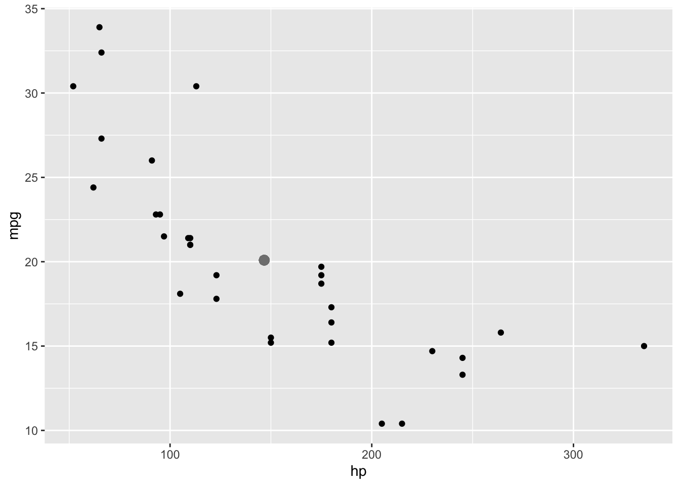
Total Sum of Squares
The total sum of squares (SST) corresponds to the sum of the squared (euclidean) distances from each point to the mean point (called the centroid). A euclidean distance is just the distance formula you learned in school: \(d=\sqrt{(y_1-y_2)^2+(x_1-x_2)^2}\) (just the hypotenuse of a triangle created by the points, from the pythagorean theorem).
ggplot(mtcars,aes(hp,mpg))+geom_point()+geom_segment(aes(x=mean(hp),y=mean(mpg), xend=hp,yend=mpg))+
  geom_point(aes(x=mean(hp),y=mean(mpg)),col='gray50',size=3)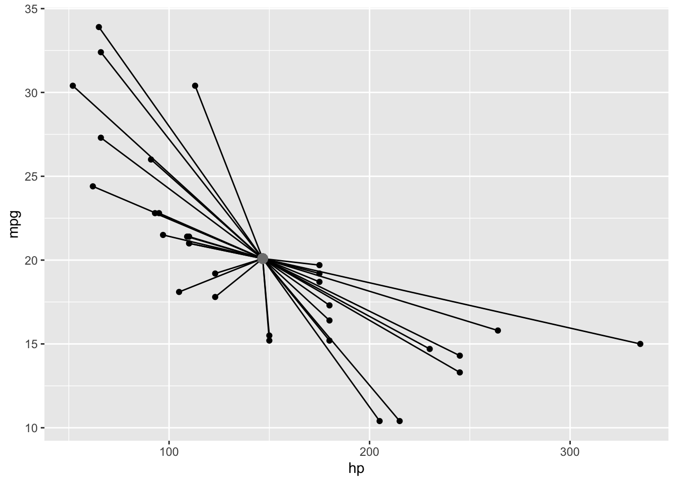
Square those distances, add them up, and you’ve got your SST!
SST<-with(mtcars, sum((hp-mean(hp))^2+(mpg-mean(mpg))^2))
SST
## [1] 146852.9One interesting equality is that the sum of the squared distances from every point to the centroid is equal to sum of the squared distances from each point to each other point, divided by the number of points
\[\sum d_{\text{i-to-centroid}}^2=\frac1N\sum d^2_{\text{i-to-j}}\]
rows<-expand.grid(1:32,1:32)
respdat<-cbind(mtcars$hp,mtcars$mpg)

temp<-cbind(respdat[rows[,1],],respdat[rows[,2],])
dists<-sqrt((temp[,1]-temp[,3])^2+(temp[,2]-temp[,4])^2)
dists<-matrix(dists,nrow=32)
dists<-dists[lower.tri(dists)]
sum(dists^2)/32
## [1] 146852.9#a shortcut using the built-in dist() function
dists<-dist(respdat,"euclid")^2
sum(dists)/32## [1] 146852.9Between-Group Sum of Squares
But what about the between-groups sum of squares (SSB)? Same idea! You just calculate how far the centroid for each group is from the grand centroid, square those distances, multiply each distance by the number of subjects in that group, and then add those numbers together
mtcars$am<-as.factor(mtcars$am)

mtcars%>%group_by(am)%>%mutate(meanhp=mean(hp),meanmpg=mean(mpg))%>%ggplot(aes(hp,mpg,color=am))+geom_point()+geom_point(aes(x=mean(hp),y=mean(mpg)),col='gray50',size=4)+geom_point(aes(meanhp,meanmpg),size=4)+geom_segment(aes(x=mean(hp),y=mean(mpg), xend=meanhp,yend=meanmpg),color='black')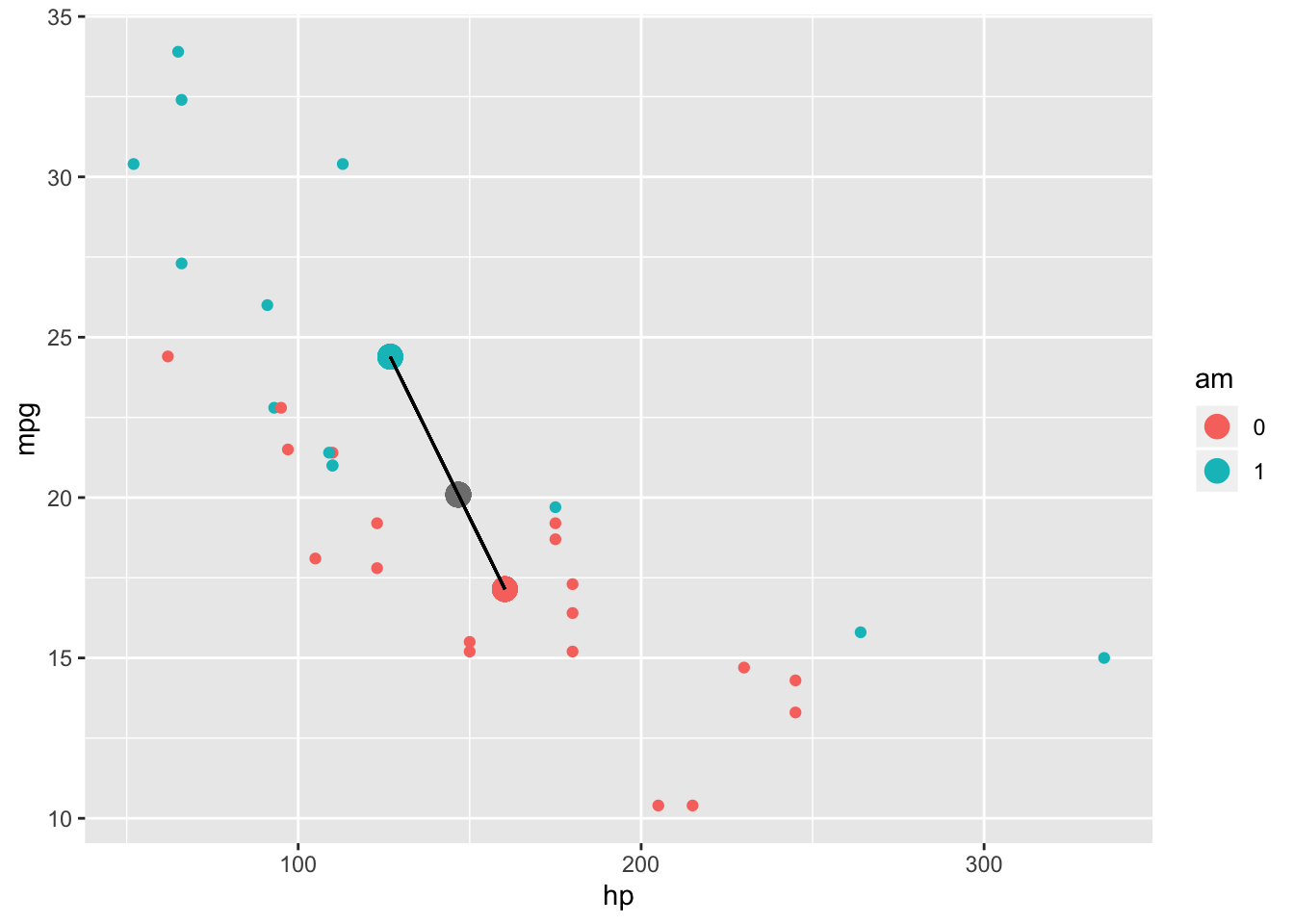
grandmean<-mtcars%>%summarize(meanhp=mean(hp),meanmpg=mean(mpg))
groupmeans<-mtcars%>%group_by(am)%>%summarize(n=n(),meanhp=mean(hp),meanmpg=mean(mpg))
SSB<-sum((cbind(groupmeans$n,groupmeans$n)*(rbind(grandmean,grandmean)-groupmeans[,-c(1,2)])^2))
SSB
## [1] 9024.649Within-Group Sum of Squares
The Sum of Squares within (SSW) is also analogous to the univariate ANOVA case. Just add up the squared distances of each subjects point in “response space” from it’s own group’s centroid
SSW<-mtcars%>%group_by(am)%>%mutate(grpmeanhp=mean(hp),grpmeanmpg=mean(mpg))%>%ungroup()%>%summarize(sum((hp-grpmeanhp)^2+(mpg-grpmeanmpg)^2))You can also just subtract the SSB from SST to find the residual SSW
SST-SSB## [1] 137828.3mtcars%>%group_by(am)%>%mutate(meanhp=mean(hp),meanmpg=mean(mpg))%>%ggplot(aes(hp,mpg,color=am))+geom_point()+
geom_point(aes(x=meanhp,y=meanmpg),size=4)+geom_segment(aes(x=hp,y=mpg,xend=meanhp,yend=meanmpg))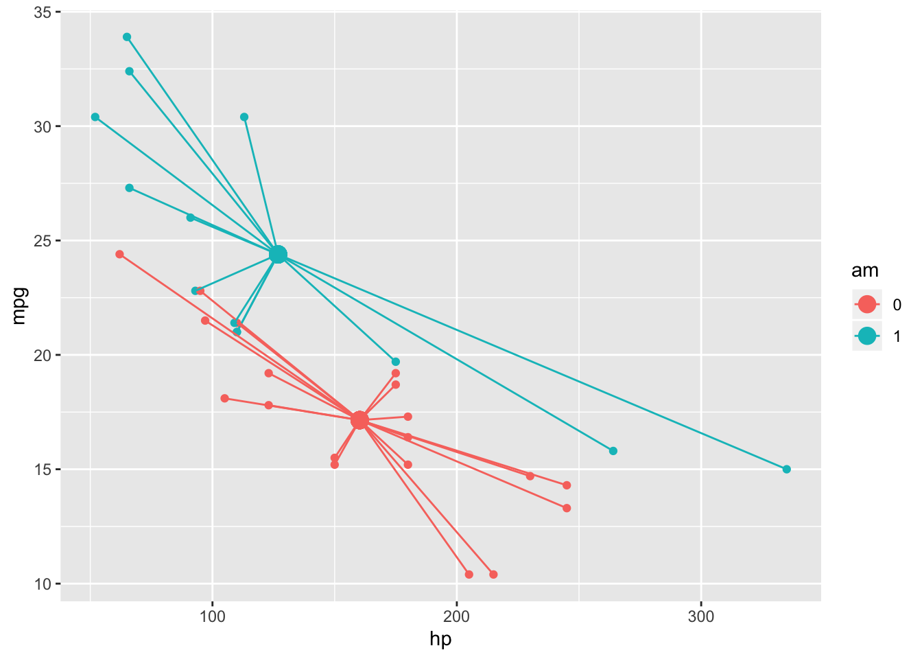
Matrix Formulation
The above helps sketch the logic of MANOVA, but rather than these sum-of-squares calculations, in practice matricies are used to compute the test statistic. These matricies are known as Sum-of-Squares-and-Cross-Products (SSCP) matricies. The sum of their diagonal elements (i.e., the trace of the matrix) gives you the sum-of-squares values we just obtained.
How do we calculate them? Each individual subject has a response vector containing their values for each of the response variables. You can subtract the mean of each response variable from each value. Then you take the outer product of each person’s centered response vector with itself, resulting in a \(p \times p\) matrix for each person, where \(p\) is the number of response variables. Just add these up across every person to get the total SSCP matrix. Recall that the outer product of a vector with itself is symmetric and calculated, for some matrix \(Z\), as follows:
\[ \mathbf{ZZ'}= \begin{pmatrix} z_1 \\ z_2 \\ \end{pmatrix} \begin{pmatrix} z_1 &z_2 \end{pmatrix} = \begin{pmatrix} z_1z_1 &z_1z_2 \\ z_1z_2 &z_2z_2 \end{pmatrix} \]
In this context, each person \(i\) has their own outer-product matrix, and we add them up to get the total
\[ \mathbf{ZZ'}= \begin{bmatrix} y_{1ij}-\bar y_{1\cdot \cdot} \\ y_{2ij}-\bar y_{2\cdot \cdot} \\ \end{bmatrix} \begin{bmatrix} y_{1ij}-\bar y_{1\cdot \cdot} &y_{2ij}-\bar y_{2\cdot \cdot} \end{bmatrix} = \begin{bmatrix} (y_{1ij}-\bar y_{1\cdot \cdot})^2 &(y_{1ij}-\bar y_{1\cdot \cdot})(y_{2ij}-\bar y_{2\cdot \cdot}) \\ (y_{1ij}-\bar y_{1\cdot \cdot}) (y_{2ij}-\bar y_{2\cdot \cdot}) & (y_{2ij}-\bar y_{2\cdot \cdot})^2 \end{bmatrix} \]
You get one of these for each person \(i\). Summing up across all people \(i\) (and groups \(j\)),
\[ \mathbf{T}=\sum_i \sum_j \begin{bmatrix}y_{1ij}-\bar y_{1\cdot \cdot}\\ y_{2ij}-\bar y_{2\cdot \cdot} \end{bmatrix}\begin{bmatrix}y_{1ij}-\bar y_{1\cdot \cdot}\\ y_{2ij}-\bar y_{2\cdot \cdot}\end{bmatrix}' \]
Here’s a way to calculate this by hand in R:
Y<-cbind(mtcars$hp,mtcars$mpg)
head(Y)
## [,1] [,2]
## [1,] 110 21.0
## [2,] 110 21.0
## [3,] 93 22.8
## [4,] 110 21.4
## [5,] 175 18.7
## [6,] 105 18.1Ycent<-cbind(Y[,1]-as.matrix(grandmean[1]),Y[,2]-as.matrix(grandmean[2]))
head(Ycent)## [,1] [,2]
## [1,] -36.6875 0.909375
## [2,] -36.6875 0.909375
## [3,] -53.6875 2.709375
## [4,] -36.6875 1.309375
## [5,] 28.3125 -1.390625
## [6,] -41.6875 -1.990625Ycent[1,]%*%t(Ycent[1,])## [,1] [,2]
## [1,] 1345.9727 -33.3626953
## [2,] -33.3627 0.8269629Tmat<-matrix(c(0,0,0,0),nrow=2)
for(i in 1:32){
Tmat<-Tmat+Ycent[i,]%*%t(Ycent[i,])
}
Tmat## [,1] [,2]
## [1,] 145726.875 -9942.694
## [2,] -9942.694 1126.047sum(diag(Tmat))## [1] 146852.9Notice that the diagonal elements of Tmat sum to SST. Furthermore, just like SST, this matrix can be partitioned into a part due to differences between groups and a part due to error. Traditionally, the part due to differences between groups (analogous to the SSB) is called the hypothesis matrix H, while the part due to error (analogous to the SSW) is called the error matrix E.
We can calculate them using a procedure similar to the one used above. For the SSE, we do the exact same thing except we center each person’s response vector using the group mean (\(\bar y_{1\cdot j}\)) rather than the grand mean (\(\bar y_{1\cdot \cdot}\))
\[\mathbf{E}=\sum_i \sum_j \begin{bmatrix}y_{1ij}-\bar y_{1\cdot j}\\ y_{2ij}-\bar y_{2\cdot j} \end{bmatrix}\begin{bmatrix}y_{1ij}-\bar y_{1\cdot j}\\ y_{2ij}-\bar y_{2\cdot j}\end{bmatrix}'\]
groupmeans<-mtcars%>%group_by(am)%>%mutate(meanhp=mean(hp), meanmpg=mean(mpg))%>%ungroup()%>%select(meanhp,meanmpg)

Ycent<-cbind(Y[,1]-as.matrix(groupmeans[,1]),Y[,2]-as.matrix(groupmeans[,2]))
head(Ycent)
## meanhp meanmpg
## [1,] -16.84615 -3.3923077
## [2,] -16.84615 -3.3923077
## [3,] -33.84615 -1.5923077
## [4,] -50.26316 4.2526316
## [5,] 14.73684 1.5526316
## [6,] -55.26316 0.9526316Ycent[1,]%*%t(Ycent[1,])## meanhp meanmpg
## [1,] 283.79290 57.14734
## [2,] 57.14734 11.50775Emat<-matrix(c(0,0,0,0),nrow=2)
for(i in 1:32){
Emat<-Emat+Ycent[i,]%*%t(Ycent[i,])
}
Emat## meanhp meanmpg
## [1,] 137107.377 -8073.9522
## [2,] -8073.952 720.8966sum(diag(Emat))## [1] 137828.3For the hypothesis matrix, it’s easier still. We need only to take the outer product of the vector containing the difference between the group mean and the grand mean for each variable and weight each entry by the number of people in that group. Since there are only two groups, we only have to add two matricies!
\[ \mathbf{E}=\sum_j n_j \begin{bmatrix}\bar y_{1\cdot \cdot}-\bar y_{1\cdot j}\\ \bar y_{2\cdot \cdot}-\bar y_{2\cdot j} \end{bmatrix}\begin{bmatrix}\bar y_{1\cdot \cdot}-\bar y_{1\cdot j}\\ \bar y_{2\cdot \cdot}-\bar y_{2\cdot j}\end{bmatrix}' \]
Ycent<-unique(groupmeans)-rbind(grandmean,grandmean)
Ycent<-as.matrix(Ycent)
Ycent
## meanhp meanmpg
## [1,] -19.84135 4.301683
## [2,] 13.57566 -2.943257#how many in each transmission group?
table(mtcars$am)##
## 0 1
## 19 13Hmat <-13*Ycent[1,]%*%t(Ycent[1,]) + 19*Ycent[2,]%*%t(Ycent[2,])
Hmat## meanhp meanmpg
## [1,] 8619.498 -1868.7415
## [2,] -1868.742 405.1506Notice first that \(T=E+H\)
Tmat## [,1] [,2]
## [1,] 145726.875 -9942.694
## [2,] -9942.694 1126.047Emat+Hmat## meanhp meanmpg
## [1,] 145726.875 -9942.694
## [2,] -9942.694 1126.047We can get these matricies straight from the manova commanda in R
summary(manova(cbind(hp,mpg)~am,data=mtcars))$SS## $am
## hp mpg
## hp 8619.498 -1868.7415
## mpg -1868.742 405.1506
##
## $Residuals
## hp mpg
## hp 137107.377 -8073.9522
## mpg -8073.952 720.8966Also, if you are more comfortable thinking in terms of covariance matricies, you can calculate the SSCPs like this
#Tmat
31*cov(cbind(mtcars$hp,mtcars$mpg))
## [,1] [,2]
## [1,] 145726.875 -9942.694
## [2,] -9942.694 1126.047#Emat
automatic<-mtcars%>%filter(am=="1")%>%select(hp,mpg)
manual<-mtcars%>%filter(am=="0")%>%select(hp,mpg)
((13-1)*cov(automatic)+(19-1)*cov(manual))## hp mpg
## hp 137107.377 -8073.9522
## mpg -8073.952 720.8966From the SSCP matricies to hypothesis tests
So we’ve got these matricies: now what? We use them to calculate test statistics! Recall that in a univariate ANOVA, an F-statistic is a ratio of the variation between groups to the variation within groups, and thus that ratio is close to 1 when those quantities are similar. Analogously, since \(\mathbf{H}\) represents the variation between groups and \(\mathbf{E}\) represents the variation within groups, then if they are very simliar we would expect \(\mathbf{H}\mathbf{E}^{-1}]\approx\mathbf{I}\), where \(\mathbf{I}\) is the identity matrix (ones along the diagonal, zeros elsewhere). The extent to which the diagonal elements of this matrix differ from ones indicate some difference in outcome variation between groups compared to that within groups, but how are we to distill that down into a test statistic?
There are four common test statistics, each of which is representable as a pseudo-F statistic. They all yield roughly the same pseudo-F.
Wilks Lambda
Wilks lambda is a common test statistic. It is calculated using the determinant of the \(\mathbf{E}\) matrix divided by the determinant of the \(\mathbf{T}\) matrix (recall that \(\mathbf{T}=\mathbf{H}+\mathbf{E}\)) \(\Lambda=\frac{|\mathbf{E}|}{|\mathbf{T}|}\). Recall that a determinant of a two-by-two matrix \(\begin{bmatrix}a & b \\ c & d \end{bmatrix}\) is just \(ad-bc\) or the difference between the product of the main diagonal and of off-diagonal.
If \(\mathbf{E}\) is large relative to \(\mathbf{T}\), then Wilks lambda will be large (thus, you reject the null hypothesis when \(\Lambda\) is close to zero).
det(Emat)/det(Tmat)## [1] 0.5158258Hotelling-Lawley
This one is a little different. Here we multiply the hypothesis matrix \(\mathbf{H}\) by the inverse of the error matrix \(\mathbf{E}\) (similar to division with scalars), and then take the trace of the resulting matrix (i.e., the sum of the diagonals). Because multiplying by the inverse of a matrix is analogous to dividing by that matrix, if \(\mathbf{H}\) is large relative to \(\mathbf{E}\), then \(T^2_0=trace(\mathbf{\mathbf{HE}^{-1}})\) will be large, and so large values of this statistic reject H0.
sum(diag(Hmat%*%solve(Emat)))## [1] 0.9386389Recall that for a \(2\times2\) matrix, the inverse of a matrix \(\mathbf{X}\) is just the matrix such that \(\mathbf{XX^{-1}=}\begin{bmatrix}1 & 0 \\ 0 & 1\end{bmatrix}\)
Pillai
Another trace-based method, this one simply takes the matrix ratio of \(\mathbf{H}\) to \(\mathbf{T}\) rather than \(\mathbf{H}\) to \(\mathbf{E}\): \(V=trace(\mathbf{HT^{-1}})\)
sum(diag(Hmat%*%solve(Tmat)))## [1] 0.4841742Roy’s Maximum Root
This final method takes the largest eigenvalue of the \(\mathbf{HE}^{-1}\) matrix. Recall that eigenvalues of a matrix \(\mathbf{X}\) are solutions \(\lambda\) to the equation \(\mathbf{Xv}=\lambda\mathbf{v}\). Basically, it means that there is a vector \(\mathbf{v}\) and scalars \(\lambda\) such that, when \(\mathbf{X}\) multiplies \(\mathbf{v}\), it will only scale the vector (by \(\lambda\) amount) and not rotate it. That equation will only have solutions if \(|\mathbf{X}-\lambda \mathbf{I}|=0\), where \(\mathbf{I}\) is the identity matrix. And can be used to find \(\lambda\) with a bit of algebra.
max(eigen(Hmat%*%solve(Emat))$values)## [1] 0.9386389In R
summary(manova(cbind(hp,mpg)~am,data=mtcars),test="Wilks")## Df Wilks approx F num Df den Df Pr(>F)
## am 1 0.51583 13.61 2 29 6.781e-05 ***
## Residuals 30
## ---
## Signif. codes: 0 '***' 0.001 '**' 0.01 '*' 0.05 '.' 0.1 ' ' 1summary(manova(cbind(hp,mpg)~am,data=mtcars),test="Hotelling-Lawley")## Df Hotelling-Lawley approx F num Df den Df Pr(>F)
## am 1 0.93864 13.61 2 29 6.781e-05 ***
## Residuals 30
## ---
## Signif. codes: 0 '***' 0.001 '**' 0.01 '*' 0.05 '.' 0.1 ' ' 1summary(manova(cbind(hp,mpg)~am,data=mtcars),test="Pillai")## Df Pillai approx F num Df den Df Pr(>F)
## am 1 0.48417 13.61 2 29 6.781e-05 ***
## Residuals 30
## ---
## Signif. codes: 0 '***' 0.001 '**' 0.01 '*' 0.05 '.' 0.1 ' ' 1summary(manova(cbind(hp,mpg)~am,data=mtcars),test="Roy")## Df Roy approx F num Df den Df Pr(>F)
## am 1 0.93864 13.61 2 29 6.781e-05 ***
## Residuals 30
## ---
## Signif. codes: 0 '***' 0.001 '**' 0.01 '*' 0.05 '.' 0.1 ' ' 1Each of these four statistics can be translated into an F-statistic for convenience (note that here, it’s around 13.61). In this example, they all agree, but they don’t have to. When this happens, Pillai’s trace is the most robust (note that it is the default in R’s manova function).
PERMANOVA
MANOVA is a little restrictive: it makes all of the ANOVA assumptions, and then some! It would be nice not to have to make these assumptions! This would permit us to use the technique on count data (e.g., abundances, percentage cover, frequencies, biomass), which for example would allow us answer many questions in ecology (e.g., do abundances of several bird species differ based on the tree composition of a sampling site?). We could also get around the weird multivariate statistics this way and compute familiar F-ratios. Let me show you what I mean.
We will start off with the distance matrix. This tells you how far each multivariate response is from each other. For example, how far is a single car’s \((hp_1, mpg_1)\) from another car’s \((hp_2, mpg_2)\) in the 2D plane? An easy way is to use the euclidean distance described above, \(d=\sqrt{(hp_1-hp_2)^2+(mpg_1-mpg_2)^2}\).
We use the distance matrix to calculate the pseudo F-ratio: the ratio of the variation between centroids to the variation within clusters. Note that this is the same as the ratio of the trace of \(\mathbf{H}\) to the trace of \(\mathbf{E}\).
euc_dist<-dist(mtcars[,c("hp","mpg")],method="euclid")
euc_dist_auto<-dist(mtcars[mtcars$am=="1",c("hp","mpg")],method="euclid")
euc_dist_manual<-dist(mtcars[mtcars$am=="0",c("hp","mpg")],method="euclid")

SSE<-sum(euc_dist_auto^2)/13+sum(euc_dist_manual^2)/19
SST<-sum(euc_dist^2)/32

Fstat=(SST-SSE)/(SSE/30)
Fstat
## [1] 1.964325To free ourselves from the assumption of normality, we can do a permutation test instead of using the F distribution to do a MANOVA. This technique, known as PERMANOVA, was developed by Marti Anderson of Auckland, NZ: original paper.
To do a PERMANOVA, we will shuffle our data randomly, re-compute f ratio, and repeat these two steps many times, saving the F each time. This gives us a large set of Fs that arise in a situation where there is no systematic difference between groups. All we have to do is just this null distribution and see how unusually our original F would be! If our actual F statistic is far away from the majority of the F statistics that arise in the simulationed distribution whwere there is no difference between groups, then we have evidence that our response variables differ between those groups!
In the mtcars example, we are comparing whether horsepower, milage, or both differ between cars with automatic versus manual transmissions. To generate the null distribution, we just randomly scramble the groups (automatic vs. manual) before we calculate each F statistic. We are literally just making up which hp, mpg data go with manual and which go with automatic. Thus, in the long run (after many repetitions), the two groups should have equal Fs on average. See the distribution of Fs after such a process below
set.seed(123)
perm.sampdist<-replicate(5000,{

randcars<-mtcars
randcars$am<-sample(randcars$am)

euc_dist<-dist(randcars[,c("hp","mpg")],method="euclid")
euc_dist_auto<-dist(randcars[randcars$am=="1",c("hp","mpg")],method="euclid")
euc_dist_manual<-dist(randcars[randcars$am=="0",c("hp","mpg")],method="euclid")

SSR<-sum(euc_dist_auto^2)/13+sum(euc_dist_manual^2)/19
SST<-sum(euc_dist^2)/32

(SST-SSR)/(SSR/30)
} )

mean(perm.sampdist>Fstat)
## [1] 0.1802hist(perm.sampdist,breaks=20); abline(v = Fstat,col='red')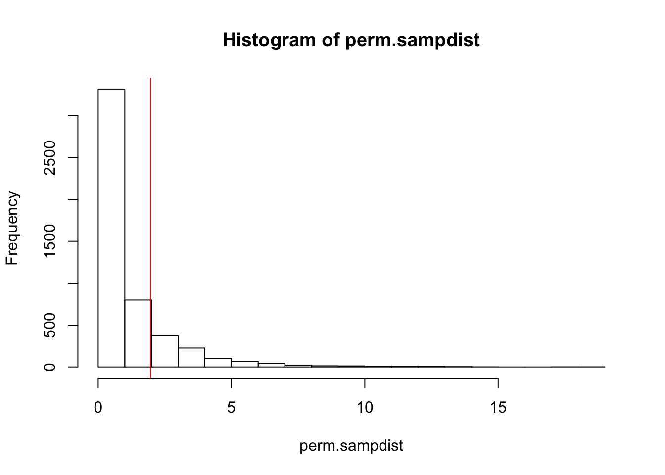
Thus, 16.88% of the simulated sampling distribution is greater than our observed F-stat. Since this distribution was created under the null hypothesis of no difference between groups, we have a nearly 17% chance of seeing an F-stat this large under the null, so we cannot reject this hypothesis as inconsistent with our data.
In the R package vegan, there is a built-in function which conducts a permanova on a distance matrix (doesn’t need to be euclidean either)!
library(vegan)
adonis(euc_dist~am,data=mtcars)
##
## Call:
## adonis(formula = euc_dist ~ am, data = mtcars)
##
## Permutation: free
## Number of permutations: 999
##
## Terms added sequentially (first to last)
##
## Df SumsOfSqs MeanSqs F.Model R2 Pr(>F)
## am 1 9025 9024.6 1.9643 0.06145 0.177
## Residuals 30 137828 4594.3 0.93855
## Total 31 146853 1.00000Note that these results are the same. However, the results do differ from those of a traditional MANOVA: making parametric assumptions does give us more power, and in this case produces significant results.
summary(manova(cbind(hp,mpg)~am,data=mtcars))## Df Pillai approx F num Df den Df Pr(>F)
## am 1 0.48417 13.61 2 29 6.781e-05 ***
## Residuals 30
## ---
## Signif. codes: 0 '***' 0.001 '**' 0.01 '*' 0.05 '.' 0.1 ' ' 1The only time the results will agree is in the univarate ANOVA case. That is to say, you can do permutational ANOVAs too, allowing you to relax assumptions. For example, assume we just want to know whether horsepower differs between cars with automatic and manual transmissions. The one-dimensional distances are simply differences between each horsepower measurement and every other. Square them all add them up and you have the total sum of squares! Divide by the number of datapoints to get your mean-squares
#parametric ANOVA
summary(aov(hp~am, mtcars))
## Df Sum Sq Mean Sq F value Pr(>F)
## am 1 8619 8619 1.886 0.18
## Residuals 30 137107 4570#permutation ANOVA
## f stat by hand
euc_dist<-dist(mtcars[,c("hp")],method="euclid")
euc_dist_auto<-dist(mtcars[mtcars$am=="1",c("hp")],method="euclid")
euc_dist_manual<-dist(mtcars[mtcars$am=="0",c("hp")],method="euclid")
SSR<-sum(euc_dist_auto^2)/13+sum(euc_dist_manual^2)/19
SST<-sum(euc_dist^2)/32
Fstat<-(SST-SSR)/(SSR/30)
## sampling distributino
perm.sampdist<-replicate(5000,{
randcars<-mtcars
randcars$am<-sample(randcars$am)
euc_dist<-dist(randcars[,c("hp")],method="euclid")
euc_dist_auto<-dist(randcars[randcars$am=="1",c("hp")],method="euclid")
euc_dist_manual<-dist(randcars[randcars$am=="0",c("hp")],method="euclid")
SSR<-sum(euc_dist_auto^2)/13+sum(euc_dist_manual^2)/19
SST<-sum(euc_dist^2)/32
(SST-SSR)/(SSR/30)
} )
mean(perm.sampdist>Fstat)## [1] 0.1784hist(perm.sampdist,breaks=20); abline(v = Fstat,col='red')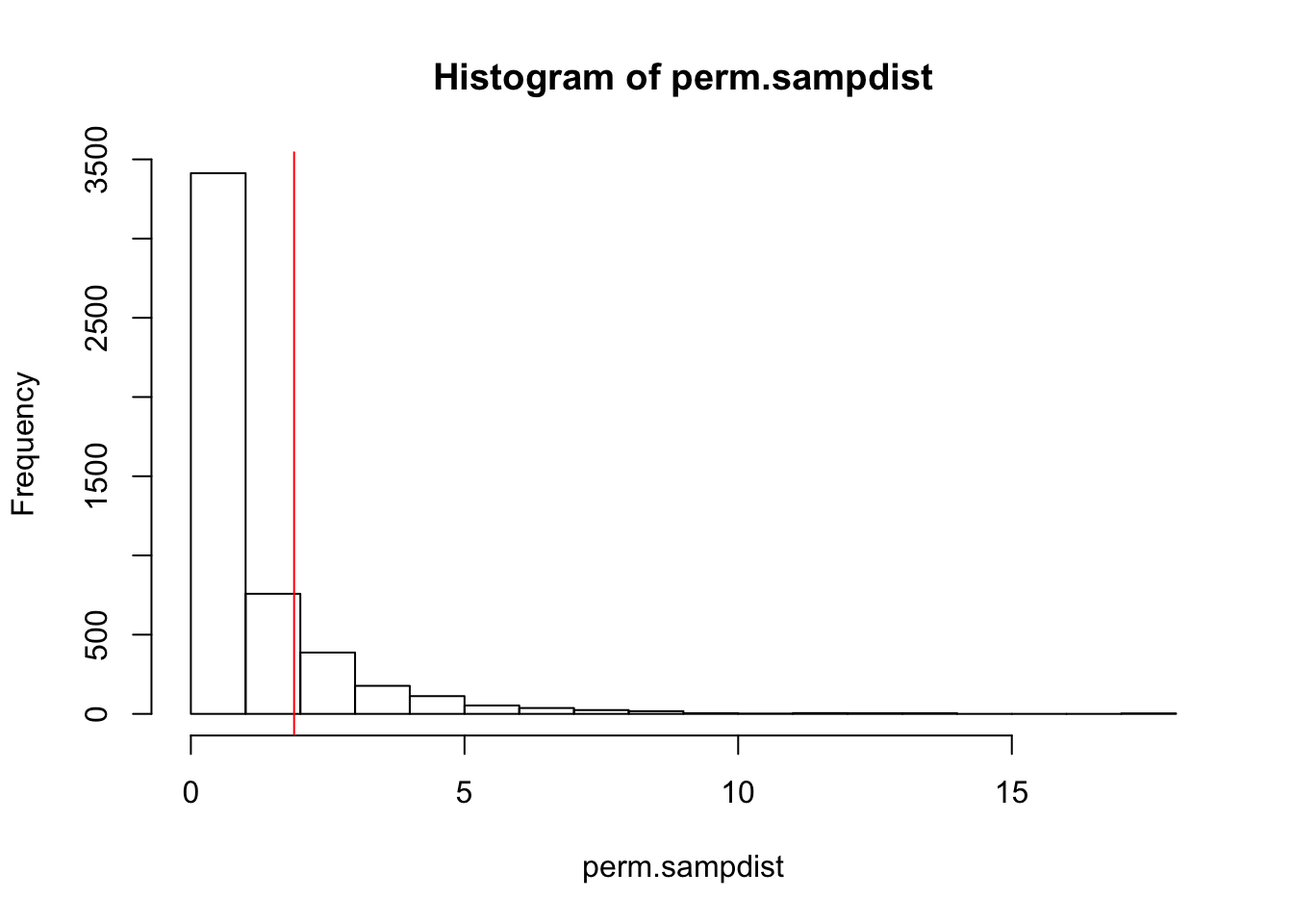
A Better Example
Now let’s do a real, more complicated example. Say we are interested in whether the presence of trees in the legume family affect the abundance of bird species. (See the following post for lots of cool additional information about this example: https://rpubs.com/collnell/manova).
The data we will use has 7 different bird species groups (columns): for each, abundance data was recorded for 32 different plots (thus, we have a 7-dimensional response variable). Also, for each of these plots, it was noted whether the trees were all part of the same species (DIVERSITY==M, for monoculture), or whether different species of trees were present (DIVERSITY==P, for polyculture). We will do a two-way PERMANOVA on this abundance data, testing whether tree diversity is associated with bird species abundance across these plots.
birds<-read.csv('https://raw.githubusercontent.com/collnell/lab-demo/master/bird_by_fg.csv')
head(birds)
## DIVERSITY PLOT CA FR GR HE IN NE OM
## 1 M 3 0 0 0 0 2 0 0
## 2 M 9 0 0 2 0 6 0 4
## 3 M 12 0 0 0 0 2 0 2
## 4 M 17 0 0 0 0 7 0 4
## 5 M 20 0 0 0 0 1 0 4
## 6 M 21 0 0 3 0 14 0 7For example, we can visualize two species at a time in two dimensions. The average abundances for both of these two species appear higher in polyclonal plots (blue dots) than in monoclonal plots (red dots):
birds1<-birds%>%group_by(DIVERSITY)%>%select(IN,OM)%>%mutate(meanIN=mean(IN),meanOM=mean(OM))%>%ungroup()%>%mutate(GmeanIN=mean(IN),GmeanOM=mean(OM))

ggplot(birds1,aes(IN,OM,color=DIVERSITY))+geom_point(aes(x=GmeanIN,y=GmeanOM),size=4,color="gray50")+geom_segment(aes(x=GmeanIN, y=GmeanOM, xend=IN, yend=OM),color="gray50",lty=2)+geom_point()+geom_point(aes(x=meanIN,y=meanOM),size=4)+geom_segment(aes(x=meanIN, y=meanOM, xend=IN, yend=OM))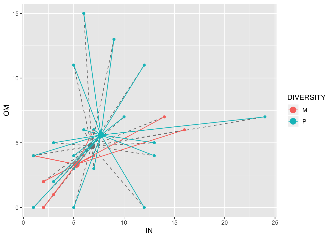
But let’s test to see if this is true: are there any differences across all 7 species? We could use euclidean distances, but it is more appropriate to use an abundance-weighted distance/dissimilarity measure like Bray-Curtis. It is a good idea to take the square (or even fourth) root of the abundance counts to minimize influential observations.
## WORKING
euc_dist<-vegdist(sqrt(birds[,-c(1:2)]),method="bray")
euc_distM<-vegdist(sqrt(birds[birds$DIVERSITY=="M",-c(1:2)]),method="bray")
euc_distP<-vegdist(sqrt(birds[birds$DIVERSITY=="P",-c(1:2)]),method="bray")

SSR<-sum(euc_distM^2)/12+sum(euc_distP^2)/20
SST<-sum(euc_dist^2)/32

Fstat<-(SST-SSR)/(SSR/30)

sum(euc_dist[1:12]^2)
## [1] 3.181082Fstat## [1] 4.158511perm.sampdist<-replicate(5000,{
randbirds<-birds
randbirds$DIVERSITY<-sample(birds$DIVERSITY)
euc_dist<-vegdist(sqrt(birds[,-c(1:2)]),method="bray")
euc_distM<-vegdist(sqrt(birds[birds$DIVERSITY=="M",-c(1:2)]),method="bray")
euc_distP<-vegdist(sqrt(birds[birds$DIVERSITY=="P",-c(1:2)]),method="bray")
SSR<-sum(euc_distM^2)/12+sum(euc_distP^2)/20
SST<-sum(euc_dist^2)/32
(SST-SSR)/(SSR/30)
} )
mean(perm.sampdist>Fstat)## [1] 0adonis(euc_dist~DIVERSITY,data=birds, method="bray")##
## Call:
## adonis(formula = euc_dist ~ DIVERSITY, data = birds, method = "bray")
##
## Permutation: free
## Number of permutations: 999
##
## Terms added sequentially (first to last)
##
## Df SumsOfSqs MeanSqs F.Model R2 Pr(>F)
## DIVERSITY 1 0.32857 0.32857 4.1585 0.12174 0.005 **
## Residuals 30 2.37033 0.07901 0.87826
## Total 31 2.69890 1.00000
## ---
## Signif. codes: 0 '***' 0.001 '**' 0.01 '*' 0.05 '.' 0.1 ' ' 1