
Hello again! In previous posts I have talked about one-way ANOVA, two-way ANOVA, and even MANOVA (for multiple response variables). But in practice, there is yet another way of partitioning the total variance in the outcome that allows you to account for repeated measures on the same subjects. These designs are very popular, but there is surpisingly little good information out there about conducting them in R. (Cue this post!)
Imagine that you have one group of subjects, and you want to test whether their heart rate is different before and after drinking a cup of coffee. Well, you would measure each person’s pulse (bpm) before the coffee, and then again after (say, five minutes after consumption). But this gives you two measurements per person, which violates the independence assumption. Thus, you would use a dependent (or paired) samples t test! In this example, the treatment (coffee) was administered within subjects: each person has a no-coffee pulse measurement, and then a coffee pulse measurement. This same treatment could have been administered between subjects (half of the sample would get coffee, the other half would not). However, you lose the each-person-acts-as-their-own-control feature and you need twice as many subjects, making it a less powerful design.
The repeated-measures ANOVA is a generalization of this idea. Imagine you had a third condition which was the effect of two cups of coffee (participants had to drink two cups of coffee and then measure then pulse). A repeated-measures ANOVA would let you ask if any of your conditions (none, one cup, two cups) affected pulse rate.
One Within-Subjects Factor
Let’s use a more realistic framing example. Say you want to know whether giving kids a pre-questions (i.e., asking them questions before a lesson), a post-questions (i.e., asking them questions after a lesson), or control (no additional practice questions) resulted in better performance on the test for that unit (out of 36 questions). Imagine that there are three units of material, the tests are normed to be of equal difficulty, and every student is in pre, post, or control condition for each three units (counterbalanced). Thus, each student gets a score from a unit where they got pre-lesson questions, a score from a unit where they got post-lesson questions, and a score from a unit where they had no additional practice questions.
Here is some data. We have 8 students (subj), factorA represents the treatment condition (within subjects; say A1 is pre, A2 is post, and A3 is control), and Y is the test score for each.
## create some data

subj<-rep(c("S1","S2","S3","S4","S5","S6","S7","S8"),3)
factorA<-rep(c("A1","A2","A3"),each=8)
Y<-c(31,33,28,35,27,22,20,24,30,28,28,31,25,23,20,25,29,20,19,33,20,18,14,17)
data<-data.frame(subj,factorA,Y)

data
## subj factorA Y
## 1 S1 A1 31
## 2 S2 A1 33
## 3 S3 A1 28
## 4 S4 A1 35
## 5 S5 A1 27
## 6 S6 A1 22
## 7 S7 A1 20
## 8 S8 A1 24
## 9 S1 A2 30
## 10 S2 A2 28
## 11 S3 A2 28
## 12 S4 A2 31
## 13 S5 A2 25
## 14 S6 A2 23
## 15 S7 A2 20
## 16 S8 A2 25
## 17 S1 A3 29
## 18 S2 A3 20
## 19 S3 A3 19
## 20 S4 A3 33
## 21 S5 A3 20
## 22 S6 A3 18
## 23 S7 A3 14
## 24 S8 A3 17table(data$factor,data$subj)##
## S1 S2 S3 S4 S5 S6 S7 S8
## A1 1 1 1 1 1 1 1 1
## A2 1 1 1 1 1 1 1 1
## A3 1 1 1 1 1 1 1 1Notice above that every subject has an observation for every level of the within-subjects factor. Now, let’s look at some means. We can get the average test score overall, we can get the average test score in each condition (i.e., each level of factor A), and we can also get the average test score for each subject.
library(dplyr)
library(tidyr)

data<-data%>%mutate(grand_mean=mean(Y))%>%
  group_by(factorA)%>%mutate(meanA=mean(Y))%>%ungroup()%>%
  group_by(subj)%>%mutate(subj_mean=mean(Y))%>%ungroup()

head(data)
## # A tibble: 6 x 6
## subj factorA Y grand_mean meanA subj_mean
## <fct> <fct> <dbl> <dbl> <dbl> <dbl>
## 1 S1 A1 31 25 27.5 30
## 2 S2 A1 33 25 27.5 27
## 3 S3 A1 28 25 27.5 25
## 4 S4 A1 35 25 27.5 33
## 5 S5 A1 27 25 27.5 24
## 6 S6 A1 22 25 27.5 21For example, the overall average test score was 25, the average test score in condition A1 (i.e., pre-questions) was 27.5, and the average test score across conditions for subject S1 was 30.
Let’s arrange the data differently by going to “wide format” with the treatment variable; we do this using the spread(key,value) command from the tidyr package.
data%>%select(subj,factorA,Y,subj_mean)%>%
  spread(factorA,Y)%>%
  select(subj,A1,A2,A3,subj_mean)%>%
  bind_rows(.,data.frame(subj="MEANS:",
                         A1=mean(Y[factorA=="A1"]),
                         A2=mean(Y[factorA=="A2"]),
                         A3=mean(Y[factorA=="A3"]),
                         subj_mean=mean(Y)))
## # A tibble: 9 x 5
## subj A1 A2 A3 subj_mean
## <chr> <dbl> <dbl> <dbl> <dbl>
## 1 S1 31 30 29 30
## 2 S2 33 28 20 27
## 3 S3 28 28 19 25
## 4 S4 35 31 33 33
## 5 S5 27 25 20 24
## 6 S6 22 23 18 21
## 7 S7 20 20 14 18
## 8 S8 24 25 17 22
## 9 MEANS: 27.5 26.2 21.2 25The last column contains each subject’s mean test score, while the bottom row contains the mean test score for each condition. The value in the bottom right corner (25) is the grand mean.
Partitioning the Total Sum of Squares (SST)
Introducing some notation, here we have \(N=8\) subjects each measured in \(K=3\) conditions. \(Y_{ij}\) is the test score for student \(i\) in condition \(j\). \(\bar Y_{\bullet j}\) is the mean test score for condition \(j\) (the means of the columns, above). \(\bar Y_{\bullet \bullet}\) is the grand mean (the average test score overall). Finally, \(\bar Y_{i\bullet}\) is the average test score for subject \(i\) (i.e., averaged across the three conditions; last column of table, above).
There are two equivalent ways to think about partitioning the sums of squares in a repeated-measures ANOVA. When you look at the table above, you notice that you break the SST into a part due to differences between conditions (SSB; variation between the three columns of factor A) and a part due to differences left over within conditions (SSW; variation within each column).
For subject \(i\) and condition \(j\), these sums of squares can be calculated as follows:
\[ SST=\sum_i^N\sum_j^K (Y_{ij}-\bar Y_{\bullet \bullet})^2 \phantom{xxxx} SSB=N\sum_j^K (\bar Y_{\bullet j}-\bar Y_{\bullet \bullet})^2 \phantom{xxxx} SSW=\sum_i^N\sum_j^K (Y_{ij}-\bar Y_{\bullet j})^2 \]
However, some of the variability within conditions (SSW) is due to variability between subjects. In the context of the example, some students might just do better on the exam than others, regardless of which condition they are in. Compare S1 and S2 in the table above, for example. Both of these students were tested in all three conditions: S1 scored an average of \(\bar Y_{1\bullet}=30\) and S2 scored an average of \(\bar Y_{2\bullet}=27\), so on average S1 scored 3 higher. We can quantify how variable students are in their average test scores (call it SSbs for sum of squares between subjects) and remove this variability from the SSW to leave the residual error (SSE). This subtraction (resulting in a smaller SSE) is what gives a repeated-measures ANOVA extra power!
\[ SSbs=K\sum_i^N (\bar Y_{i\bullet}-\bar Y_{\bullet \bullet})^2 \]
Look at the left side of the diagram below: it gives the additive relations for the sums of squares.

There is another way of looking at the \(SS\) decomposition that some find more intuitive. Starting with the \(SST\), you could instead break it into a part due to differences between subjects (the \(SSbs\) we saw before) and a part left over within subjects (\(SSws\)). The \(SSws\) is quantifies the variability of the students three test scores around their average test score, namely
\[ SSws=\sum_i^N\sum_j^K (\bar Y_{ij}-\bar Y_{i \bullet})^2 \]
This calculation is analogous to the SSW calculation, except it is done within subjects/rows (with row means) instead of within conditions/columns (with column means).
Now, the variability within subjects’ test scores is clearly due in part to the effect of the condition (i.e., \(SSB\)). That is, the reason a students outcome would differ for each of the three time points include the effect of the treatment itself (\(SSB\)) and error (\(SSE\)). If we subtract this from the variability within subjects (i.e., if we do \(SSws-SSB\)) then we get the \(SSE\).
Let’s calculate these sums of squares using R. Notice that in the original data frame (data), I have used mutate() to create new columns that contain each of the means of interest in every row. By doing operations on these mean columns, this keeps me from having to multiply by \(K\) or \(N\) when performing sums of squares calculations in R. You can do them however you want, but I find this to be quicker. See if you
data%>%summarize( SST =  sum( (Y - grand_mean)^2 ),
                  SSB =  sum( (meanA - grand_mean)^2 ),
                  SSW =  sum( (Y - meanA)^2 ),
                  SSbs = sum( (subj_mean - grand_mean)^2 ),
                  SSws = sum( (Y - subj_mean)^2 ),
                  SSE =  SSws-SSB)
## # A tibble: 1 x 6
## SST SSB SSW SSbs SSws SSE
## <dbl> <dbl> <dbl> <dbl> <dbl> <dbl>
## 1 756 175 581 504 252 77Notice that
\[ \begin{aligned} SST&=SSB+SSW\\ &=SSB+SSbs+SSE\\ &=SSbs+SSws\\ &=SSbs+SSB+SSE \end{aligned} \]
The degrees of freedom calculations are very similar to one-way ANOVA. If \(K\) is the number of conditions and \(N\) is the number of subjects, $
\[ DF_B=K-1, DF_W=DF_{ws}=K(N-1),DF_{bs}=N-1,$ and $DD_E=(K-1)(N-1) \]
Just like in a regular one-way ANOVA, we are looking for a ratio of the variance between conditions to error (or noise) within each condition. The only difference is, we have to remove the variation due to subjects first. Once we have done so, we can find the \(F\) statistic as usual,
\[F=\frac{SSB/DF_B}{SSE/DF_E}=\frac{175/(3-1)}{77/[(3-1)(8-1)]}=\frac{175/2}{77/14}=87.5/5.5=15.91\]
Under the null hypothesis of no treatment effect, we expect \(F\) statistics to follow an \(F\) distribution with 2 and 14 degrees of freedom. Assuming this is true, what is the probability of observing an \(F\) at least as big as the one we got?
Fstat <- (175/2)/(77/14)

pf(Fstat, df1 = 2, df2 = 14, lower.tail = F)
## [1] 0.0002486745plot(curve(df(x,2,14),from=0, to=20), type="line")
abline(v=Fstat,h=0,add=T)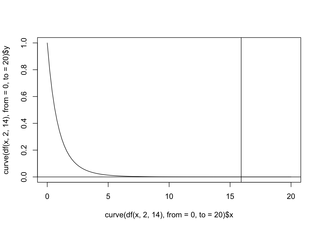
Wow, looks very unusual to see an \(F\) this big if the treatment has no effect! Let’s confirm our calculations by using the repeated-measures ANOVA function in base R. Notice that you must specify the error term yourself. It will always be of the form Error(unit with repeated measures/ within-subjects variable). Take a minute to confirm the correspondence between the table below and the sum of squares calculations above.
anova1<-aov(Y ~ factorA + Error(subj/factorA), data=data)
summary(anova1)
##
## Error: subj
## Df Sum Sq Mean Sq F value Pr(>F)
## Residuals 7 504 72
##
## Error: subj:factorA
## Df Sum Sq Mean Sq F value Pr(>F)
## factorA 2 175 87.5 15.91 0.000249 ***
## Residuals 14 77 5.5
## ---
## Signif. codes: 0 '***' 0.001 '**' 0.01 '*' 0.05 '.' 0.1 ' ' 1Naive analysis (not accounting for repeated measures)
Look what happens if we do not account for the fact that some of the variability within conditions is due to variability between subjects.
summary(aov(Y ~ factorA, data=data))## Df Sum Sq Mean Sq F value Pr(>F)
## factorA 2 175 87.50 3.163 0.063 .
## Residuals 21 581 27.67
## ---
## Signif. codes: 0 '***' 0.001 '**' 0.01 '*' 0.05 '.' 0.1 ' ' 1Notice that this regular one-way ANOVA uses \(SSW\) as the denominator sum of squares (the error), and this is much bigger than it would be if you removed the \(SSbs\). Notice that the numerator (the between-groups sum of squares, SSB) does not change. Thus, by not correcting for repeated measures, we are not only violating the independence assumption, we are leaving lots of error on the table: indeed, this extra error increases the denominator of the F statistic to such an extent that it masks the effect of treatment!
Mixed-effects model of same data
You can also achieve the same results using a hierarchical model with the lme4 package in R. This is what I normally use in practice.
library(lme4)

options(contrasts = c("contr.treatment","contr.poly"))

fit_fixed<-lm(Y~factorA+subj,data=data)
fit_random<-lmer(Y ~ factorA + (1|subj), data=data)

anova(fit_fixed)
## Analysis of Variance Table
##
## Response: Y
## Df Sum Sq Mean Sq F value Pr(>F)
## factorA 2 175 87.5 15.909 0.0002487 ***
## subj 7 504 72.0 13.091 3.572e-05 ***
## Residuals 14 77 5.5
## ---
## Signif. codes: 0 '***' 0.001 '**' 0.01 '*' 0.05 '.' 0.1 ' ' 1anova(fit_random)## Analysis of Variance Table
## Df Sum Sq Mean Sq F value
## factorA 2 175 87.5 15.909Notice that it doesn’t matter whether you model subjects as fixed effects or random effects: your test of factor A is equivalent in both cases.
If you ask for summary(fit) you will get the regression output. The (intercept) is giving you the mean for group A1 and testing whether it is equal to zero, while the FactorAA2 and FactorAA3 coefficient estimates are testing the differences in means between each of those two groups again the mean of A1. Notice that this is equivalent to doing post-hoc tests for a repeated measures ANOVA (you can get the same results from the emmeans package).
summary(fit_random)## Linear mixed model fit by REML ['lmerMod']
## Formula: Y ~ factorA + (1 | subj)
## Data: data
##
## REML criterion at convergence: 119.6
##
## Scaled residuals:
## Min 1Q Median 3Q Max
## -1.32066 -0.45009 -0.09031 0.19543 1.85958
##
## Random effects:
## Groups Name Variance Std.Dev.
## subj (Intercept) 22.17 4.708
## Residual 5.50 2.345
## Number of obs: 24, groups: subj, 8
##
## Fixed effects:
## Estimate Std. Error t value
## (Intercept) 27.500 1.860 14.788
## factorAA2 -1.250 1.173 -1.066
## factorAA3 -6.250 1.173 -5.330
##
## Correlation of Fixed Effects:
## (Intr) fctAA2
## factorAA2 -0.315
## factorAA3 -0.315 0.500library(emmeans)
emmeans(anova1,~factorA)%>%pairs()## contrast estimate SE df t.ratio p.value
## A1 - A2 1.25 1.17 14 1.066 0.5496
## A1 - A3 6.25 1.17 14 5.330 0.0003
## A2 - A3 5.00 1.17 14 4.264 0.0021
##
## P value adjustment: tukey method for comparing a family of 3 estimatesChecking Assumptions
Ah yes, assumptions. We should have done this earlier, but here we are. Just as typical ANOVA makes the assumption that groups have equal population variances, repeated-measures ANOVA makes a variance assumption too, called sphericity.
This assumption is about the variances of the response variable in each group, or the covariance of the response variable in each pair of groups. A stricter assumption than sphericity, but one that helps to understand it, is called compound symmetery. Compound symmetry holds if all covariances are equal and all variances are equal. Here’s what I mean. Look at the data below. Compound symmetry assumes that \(var(A1)=var(A2)=var(A3)\) and that \(cov(A1,A2)=cov(A1,A2)=cov(A2,A3)\). We can begin to assess this by eyeballing the variance-covariance matrix.
wideY<-data%>%select(subj,Y,factorA)%>%spread(factorA,Y)%>%select(-1)
wideY
## # A tibble: 8 x 3
## A1 A2 A3
## <dbl> <dbl> <dbl>
## 1 31 30 29
## 2 33 28 20
## 3 28 28 19
## 4 35 31 33
## 5 27 25 20
## 6 22 23 18
## 7 20 20 14
## 8 24 25 17cov(wideY,wideY)## A1 A2 A3
## A1 28.28571 18.42857 27.85714
## A2 18.42857 13.64286 20.21429
## A3 27.85714 20.21429 41.07143Here it looks like A3 has a larger variance than A2, which in turn has a larger variance than A1. Also, the covariance between A1 and A3 is greater than the other two covariances. Fortunately, we do not have to satisfy compound symmetery! We have to satisfy a lower bar: sphericity. However, if compound symmetry is met, then sphericity will also be met.
In brief, we assume that the variance all pairwise differences are equal across conditions. That is, we subtract each students’ scores in condition A1 from their scores in condition A2 (i.e., \(A1-A2\)) and calculate the variance of these differences. We do the same thing for \(A1-A3\) and \(A2-A3\). Below, we convert the data to wide format (wideY, below), overwrite the original columns with the difference columns using transmute(), and then append the variances of these columns with bind_rows()
wideY%>%transmute(`A1-A2`=A1-A2, `A1-A3`=A1-A3, `A2-A3`=A2-A3)%>%bind_rows(summarize_all(., .funs = var))## # A tibble: 9 x 3
## `A1-A2` `A1-A3` `A2-A3`
## <dbl> <dbl> <dbl>
## 1 1 2 1
## 2 5 13 8
## 3 0 9 9
## 4 4 2 -2
## 5 2 7 5
## 6 -1 4 5
## 7 0 6 6
## 8 -1 7 8
## 9 5.07 13.6 14.3We can also get these variances-of-differences straight from the covariance matrix using the identity \(Var(X-Y)=Var(X)+Var(Y)-2Cov(X,Y)\). For example, \(Var(A1-A2)=Var(A1)+Var(A2)-2Cov(A1,A2)=28.286+13.643-2(18.429)=5.071\)
Notice that the variance of A1-A2 is small compared to the other two. But these are sample variances based on a small sample! We can use them to formally test whether we have enough evidence in our sample to reject the null hypothesis that the variances are equal in the population.
To do this, we can use Mauchly’s test of sphericity. If \(p<.05\), then we reject the null hypothesis of sphericity (i.e., the assumption is violated); if not, we are in the clear. To do this, we will use the Anova() function in the car package. We need to create a model object from the wide-format outcome data (model), define the levels of the independent variable (A), and then specify the ANOVA as we do below.
library(car)

#use the wide data from before to build a model
model<-lm(as.matrix(wideY)~1)

#define the within-subjects factor
A<-factor(c("A1","A2","A3"))

aov1<-Anova(model,idata=data.frame(A),idesign=~A)
summary(aov1)
##
## Type III Repeated Measures MANOVA Tests:
##
## ------------------------------------------
##
## Term: (Intercept)
##
## Response transformation matrix:
## (Intercept)
## A1 1
## A2 1
## A3 1
##
## Sum of squares and products for the hypothesis:
## (Intercept)
## (Intercept) 45000
##
## Multivariate Tests: (Intercept)
## Df test stat approx F num Df den Df Pr(>F)
## Pillai 1 0.967492 208.3333 1 7 1.8258e-06 ***
## Wilks 1 0.032508 208.3333 1 7 1.8258e-06 ***
## Hotelling-Lawley 1 29.761905 208.3333 1 7 1.8258e-06 ***
## Roy 1 29.761905 208.3333 1 7 1.8258e-06 ***
## ---
## Signif. codes: 0 '***' 0.001 '**' 0.01 '*' 0.05 '.' 0.1 ' ' 1
##
## ------------------------------------------
##
## Term: A
##
## Response transformation matrix:
## A1 A2
## A1 1 0
## A2 0 1
## A3 -1 -1
##
## Sum of squares and products for the hypothesis:
## A1 A2
## A1 312.5 250
## A2 250.0 200
##
## Multivariate Tests: A
## Df test stat approx F num Df den Df Pr(>F)
## Pillai 1 0.766667 9.857143 2 6 0.012704 *
## Wilks 1 0.233333 9.857143 2 6 0.012704 *
## Hotelling-Lawley 1 3.285714 9.857143 2 6 0.012704 *
## Roy 1 3.285714 9.857143 2 6 0.012704 *
## ---
## Signif. codes: 0 '***' 0.001 '**' 0.01 '*' 0.05 '.' 0.1 ' ' 1
##
## Univariate Type III Repeated-Measures ANOVA Assuming Sphericity
##
## Sum Sq num Df Error SS den Df F value Pr(>F)
## (Intercept) 15000 1 504 7 208.333 1.826e-06 ***
## A 175 2 77 14 15.909 0.0002487 ***
## ---
## Signif. codes: 0 '***' 0.001 '**' 0.01 '*' 0.05 '.' 0.1 ' ' 1
##
##
## Mauchly Tests for Sphericity
##
## Test statistic p-value
## A 0.70838 0.35547
##
##
## Greenhouse-Geisser and Huynh-Feldt Corrections
## for Departure from Sphericity
##
## GG eps Pr(>F[GG])
## A 0.77422 0.0009751 ***
## ---
## Signif. codes: 0 '***' 0.001 '**' 0.01 '*' 0.05 '.' 0.1 ' ' 1
##
## HF eps Pr(>F[HF])
## A 0.9527163 0.0003306405Mauchly’s test has a \(p=.355\), so we fail to reject the sphericity hypothesis (we are good to go)! In cases where sphericity is violated, you can use a significance test that corrects for this (either Greenhouse-Geisser or Huynh-Feldt).
Notice that we have specifed multivariate=F as an argument to the summary function. By default, the summary will give you the results of a MANOVA treating each of your repeated measures as a different response variable. This isn’t really useful here, because the groups are defined by the single within-subjects variable.
Effect size
You can compute eta squared (\(\eta^2\)) just as you would for a regular ANOVA: it’s just the proportion of total variation due to the factor of interest. Here, there is just a single factor, so \(\eta^2=\frac{SSB}{SST}=\frac{175}{756}=.2315\)
One between, one within (a two-way split plot design)
Now, let’s take the same data, but let’s add a between-subjects variable to it. Let’s say subjects S1, S2, S3, and S4 are in one between-subjects condition (e.g., female; call it B1) while subjects S5, S6, S7, and S8 are in another between-subjects condition (e.g., male; call it B2).
###### One between, one within (Two-way split plot)

subj<-rep(c("S1","S2","S3","S4","S5","S6","S7","S8"),3)
factorA<-rep(c("A1","A2","A3"),each=8)
factorB<-rep(rep(c("B1","B2"),each=4),3)
Y<-c(31,33,28,35,27,22,20,24,30,28,28,31,25,23,20,25,29,20,19,33,20,18,14,17)
data<-data.frame(subj,factorA,factorB,Y)
data
## subj factorA factorB Y
## 1 S1 A1 B1 31
## 2 S2 A1 B1 33
## 3 S3 A1 B1 28
## 4 S4 A1 B1 35
## 5 S5 A1 B2 27
## 6 S6 A1 B2 22
## 7 S7 A1 B2 20
## 8 S8 A1 B2 24
## 9 S1 A2 B1 30
## 10 S2 A2 B1 28
## 11 S3 A2 B1 28
## 12 S4 A2 B1 31
## 13 S5 A2 B2 25
## 14 S6 A2 B2 23
## 15 S7 A2 B2 20
## 16 S8 A2 B2 25
## 17 S1 A3 B1 29
## 18 S2 A3 B1 20
## 19 S3 A3 B1 19
## 20 S4 A3 B1 33
## 21 S5 A3 B2 20
## 22 S6 A3 B2 18
## 23 S7 A3 B2 14
## 24 S8 A3 B2 17table(data$factorA,data$subj)##
## S1 S2 S3 S4 S5 S6 S7 S8
## A1 1 1 1 1 1 1 1 1
## A2 1 1 1 1 1 1 1 1
## A3 1 1 1 1 1 1 1 1table(data$factorB,data$subj)##
## S1 S2 S3 S4 S5 S6 S7 S8
## B1 3 3 3 3 0 0 0 0
## B2 0 0 0 0 3 3 3 3You can see from the tabulation that every level of factor A has an observation for each student (thus, it is fully within-subjects), while factor B does not (students are either in one level of factor B or the other, making it a between-subjects variable).
data<-data%>%mutate(grand_mean=mean(Y))%>%
  group_by(factorA,factorB)%>%mutate(meanAB=mean(Y))%>%ungroup()%>%
  group_by(factorA)%>%mutate(meanA=mean(Y))%>%ungroup()%>%
  group_by(factorB)%>%mutate(meanB=mean(Y))%>%ungroup()%>%
  group_by(subj)%>%mutate(subj_mean=mean(Y))%>%
  ungroup()

data
## # A tibble: 24 x 9
## subj factorA factorB Y grand_mean meanAB meanA meanB subj_mean
## <fct> <fct> <fct> <dbl> <dbl> <dbl> <dbl> <dbl> <dbl>
## 1 S1 A1 B1 31 25 31.8 27.5 28.8 30
## 2 S2 A1 B1 33 25 31.8 27.5 28.8 27
## 3 S3 A1 B1 28 25 31.8 27.5 28.8 25
## 4 S4 A1 B1 35 25 31.8 27.5 28.8 33
## 5 S5 A1 B2 27 25 23.2 27.5 21.2 24
## 6 S6 A1 B2 22 25 23.2 27.5 21.2 21
## 7 S7 A1 B2 20 25 23.2 27.5 21.2 18
## 8 S8 A1 B2 24 25 23.2 27.5 21.2 22
## 9 S1 A2 B1 30 25 29.2 26.2 28.8 30
## 10 S2 A2 B1 28 25 29.2 26.2 28.8 27
## # … with 14 more rowsSame as before, we will use these group means to calculate sums of squares. Since we have two factors, it no longer makes sense to talk about sum of squares between conditions and within conditions (since we have to sets of conditions to keep separate). Thus, a notation change is necessary: let \(SSA\) refer to the between-groups sum of squares for factor A and let \(SSB\) refer to the between groups sum of squares for factor B. (Notice, perhaps confusingly, that \(SSB\) used to refer to what we are now calling \(SSA\)).
To keep things somewhat manageable, let’s start by partitioning the \(SST\) into between-subjects and within-subjects variability (\(SSws\) and \(SSbs\), respectively). Now, variability within subjects can be broken down into the variation due to the within-subjects factor A (\(SSA\)), the interaction sum of squares \(SSAB\), and the residual error \(SSE\). The between-subjects sum of squares \(SSbs\) can be decomposed into an effect of the between-subjects variable (\(SSB\)) and the leftover noise within each between-subjects level (i.e., how far each subject’s mean is from the mean for the between-subjects factor, squared, and summed up).

The sums of squares calculations are defined as above, except we are introducing a couple new ones. Let’s write the test score for student \(i\) in level \(j\) of factor A and level \(k\) of factor B as \(Y_{ijk}\). The mean test score for student \(i\) is denoted \(\bar Y_{i\bullet \bullet}\). The mean test score for a student in level \(j\) of factor A and level \(k\) of factor by is denoted \(\bar Y_{\bullet jk}\). The mean test score for level \(j\) of factor A is denoted \(\bar Y_{\bullet j \bullet}\), and the mean score for level \(k\) of factor B is \(\bar Y_{\bullet \bullet k}\).
Two of these we havent seen before: \(SSs(B)\) and \(SSAB\). Let’s have a look at their formulas. The first is the sum of squared deviations of subject means around their group mean for the between-groups factor (factor B):
\[ SSs(B)=n_A\sum_i\sum_k (\bar Y_{i\bullet \bullet}-\bar Y_{\bullet \bullet k})^2 \]
It’s kind of like SSB, but treating subject mean as a factor mean and factor B mean as a grand mean. It quantifies the amount of variability in each group of the between-subjects factor. Here, \(n_A\) is the number of people in each group of factor A (here, 8)
Then we have this one:
\[ \begin{aligned} SS_{AB}&=n_{AB}\sum_i\sum_j\sum_k(\text{cellmean - (grand mean + effect of }A_j + \text{effect of }B_k ))^2 \\ &=n_{AB}\sum\sum\sum(\bar Y_{\bullet jk} - (\bar Y_{\bullet \bullet \bullet} + (\bar Y_{\bullet j \bullet} - \bar Y_{\bullet \bullet \bullet}) + (\bar Y_{\bullet \bullet k}-\bar Y_{\bullet \bullet \bullet}) ))^2 \\ &=n_{AB}\sum\sum\sum(\bar Y_{\bullet jk} - (\bar Y_{\bullet j \bullet} + \bar Y_{\bullet \bullet k} - \bar Y_{\bullet \bullet \bullet}) ))^2 \\ &=n_{AB}\sum\sum\sum(\bar Y_{\bullet jk} - \bar Y_{\bullet j \bullet} - \bar Y_{\bullet \bullet k} + \bar Y_{\bullet \bullet \bullet} ))^2 \\ \end{aligned} \] Where \(N_{AB}\) is the number of responses each cell, assuming cell sizes are equal.
This formula is interesting. It says, take the grand mean… now add the effect of being in level \(j\) of factor A (i.e., how much higher/lower than the grand mean is it?)…now add the effect of being in level \(k\) of factor B (i.e., how much higher/lower than the grand mean is it?). Now, that’s what we would expect the cell mean to be if there was no interaction (only the separate, additive effects of factors A and B). To find how much of each cell is due to the interaction, you look at how far the cell mean is from this expected value. If it is zero, for instance, then that cell contributes nothing to the interaction sum of squares.
Let’s do a quick example. The grand mean is \(\bar Y_{\bullet \bullet \bullet}=25\). The mean test score for group B1 is \(\bar Y_{\bullet \bullet 1}=28.75\), which is \(3.75\) above the grand mean (this is the effect of being in group B1); for group B2 it is \(\bar Y_{\bullet \bullet 2}=21.25\), which is .375 lower than the grand mean (effect of group B2). The means for the within-subjects factor are the same as before: \(\bar Y_{\bullet 1 \bullet}=27.5\), \(\bar Y_{\bullet 2 \bullet}=23.25\), \(\bar Y_{\bullet 3 \bullet}=17.25\). Subtracting the grand mean gives the effect of each condition: A1 effect$ = +2.5$, A2 effect \(= +1.25\), A3 effect \(= -3.75\).
So if you are in condition A1 and B1, with no interaction we expect the cell mean to be \(\text{grand mean + effect of A1 + effect of B1}=25+2.5+3.75=31.25\). However, the actual cell mean for cell A1,B1 (i.e., the average of the test scores for the four observations in that condtion) is \(\bar Y_{\bullet 1 1}=\frac{31+33+28+35}{4}=31.75\). Thus, the interaction effect for cell A1,B1 is the difference between 31.75 and the expected 31.25, or 0.5. Do this for all six cells, square them, and add them up, and you have your interaction sum of squares! If this is big enough, you will be able to reject the null hypothesis of no interaction!

All of the required means are illustrated in the table above. I think it is a really helpful way to think about it (columns are the within-subjects factor A, small rows are each individual students, grouped into to larger rows representing the two levels of the between-subjects factor).
Let’s use these means to calculate the sums of squares in R:
data%>%summarize(SST=sum((Y-grand_mean)^2),
                 SSA=sum((meanA-grand_mean)^2),
                 SSB=sum((meanB-grand_mean)^2),
                 SSbs=sum((subj_mean-grand_mean)^2),
                 `SSs(B)`=sum((subj_mean-meanB)^2),
                 SSW=sum((Y-meanB)^2),
                 SSAB=sum((meanAB+grand_mean-meanA-meanB)^2),
                 SScells=sum((Y-meanAB)^2),
                 SSws=sum((Y-subj_mean)^2),
                 SSres=sum((Y-subj_mean-meanAB+meanB)^2))
## # A tibble: 1 x 10
## SST SSA SSB SSbs `SSs(B)` SSW SSAB SScells SSws SSres
## <dbl> <dbl> <dbl> <dbl> <dbl> <dbl> <dbl> <dbl> <dbl> <dbl>
## 1 756 175 338. 504 166. 418. 7 236. 252 70Wow, OK. We’ve got a lot here. We want to do three \(F\) tests: the effect of factor A, the effect of factor B, and the effect of the interaction. Notice in the sum-of-squares partitioning diagram above that for factor B, the error term is \(SSs(B)\), so we do \(F=\frac{SSB/DF_B}{SSs(B)/DF_{s(B)}}\). Degrees of freedom for SSB are same as before: number of levels of that factor (2) minus one, so \(DF_B=1\). We can see from the diagram that \(DF_{bs}=DF_B+DF_{s(B)}\), and we know \(DF_{bs}=8-1=1\), so \(DF_{s(B)}=7-1=6\). (A shortcut to remember is \(DF_{bs}=N-B=8-2=6\), where \(N\) is the number of subjects and \(B\) is the number of levels of factor B. Therefore, our F statistic is \(F=F=\frac{337.5}{166.5/6}=12.162\), a large F statistic! This would be very unusual if the null hypothesis of no effect were true (we would expect Fs around 1); thus, we reject the null hypothesis: we have evidence that there is an effect of the between-subjects factor (e.g., sex of student) on test score.
#pvalue
pf(12.162, df1 = 1, df2 = 6,lower.tail = F)
## [1] 0.01302444How about factor A? Well, as before \(F=\frac{SSA/DF_A}{SSE/DF_E}\). The degrees of freedom for factor A is just \(A-1=3-1=2\), where \(A\) is the number of levels of factor A. To get \(DF_E\), we do \((A-1)(N-B)=(3-1)(8-2)=12\). So we have for our F statistic \(F=\frac{MSA}{MSE}=\frac{175/2}{70/12}=15\), a very large F statistic! Thus, we reject the null hypothesis that factor A has no effect on test score.
#pvalue
pf(15, df1 = 2, df2 = 15,lower.tail = F)
## [1] 0.0002639919Finally, what about the interaction? We will use the same denominator as in the above F statistic, but we need to know the numerator degrees of freedom (i.e., for the interaction). We can calculate this as \(DF_{A\times B}=(A-1)(B-1)=2\times1=2\). So our test statistic is \(F=\frac{MS_{A\times B}}{MSE}=\frac{7/2}{70/12}=0.6\), no significant interaction
#pvalue
pf(.6, df1 = 2, df2 = 12,lower.tail = F)
## [1] 0.5644739Let’s see how our manual calculations square with the repeated measures ANOVA output in R
summary(aov(Y ~ factorA*factorB + Error(subj/factorA), data=data))##
## Error: subj
## Df Sum Sq Mean Sq F value Pr(>F)
## factorB 1 337.5 337.5 12.16 0.013 *
## Residuals 6 166.5 27.8
## ---
## Signif. codes: 0 '***' 0.001 '**' 0.01 '*' 0.05 '.' 0.1 ' ' 1
##
## Error: subj:factorA
## Df Sum Sq Mean Sq F value Pr(>F)
## factorA 2 175 87.50 15.0 0.000544 ***
## factorA:factorB 2 7 3.50 0.6 0.564474
## Residuals 12 70 5.83
## ---
## Signif. codes: 0 '***' 0.001 '**' 0.01 '*' 0.05 '.' 0.1 ' ' 1Perfect!
Let’s look at the mixed model output to see which means differ
fit<-lmer(Y~factorA*factorB+(1|subj), data=data)

#same results as above
anova(fit)
## Analysis of Variance Table
## Df Sum Sq Mean Sq F value
## factorA 2 175.000 87.500 15.000
## factorB 1 70.946 70.946 12.162
## factorA:factorB 2 7.000 3.500 0.600summary(fit)## Linear mixed model fit by REML ['lmerMod']
## Formula: Y ~ factorA * factorB + (1 | subj)
## Data: data
##
## REML criterion at convergence: 100.5
##
## Scaled residuals:
## Min 1Q Median 3Q Max
## -1.60145 -0.33198 -0.07118 0.41404 1.81904
##
## Random effects:
## Groups Name Variance Std.Dev.
## subj (Intercept) 7.306 2.703
## Residual 5.833 2.415
## Number of obs: 24, groups: subj, 8
##
## Fixed effects:
## Estimate Std. Error t value
## (Intercept) 31.750 1.812 17.518
## factorAA2 -2.500 1.708 -1.464
## factorAA3 -6.500 1.708 -3.806
## factorBB2 -8.500 2.563 -3.316
## factorAA2:factorBB2 2.500 2.415 1.035
## factorAA3:factorBB2 0.500 2.415 0.207
##
## Correlation of Fixed Effects:
## (Intr) fctAA2 fctAA3 fctBB2 fAA2:B
## factorAA2 -0.471
## factorAA3 -0.471 0.500
## factorBB2 -0.707 0.333 0.333
## fctrAA2:BB2 0.333 -0.707 -0.354 -0.471
## fctrAA3:BB2 0.333 -0.354 -0.707 -0.471 0.500Since A1,B1 is the reference category (e.g., female students in the pre-question condition), the estimates are differences in means compared to this group, and the significance tests are t tests (not corrected for multiple comparisons). For example, female students (i.e., B1, the reference) in the post-question condition (i.e., A3) did 6.5 points worse on average, and this difference is significant (p=.0025). However, for female students (B1) in the pre-question condition (i.e., A2), while they did 2.5 points worse on average, this difference was not significant (p=.1690). Male students (i.e., B2) in the pre-question condition (the reference category, A1), did 8.5 points worse on average than female students in the same category, a significant difference (p=.0068). And so on (the interactions compare the mean score boys in A2 and A3 with the mean for girls in A1).
We can visualize these using an interaction plot!
library(ggplot2)
data%>%ggplot(aes(y=meanAB, x=factorA, color=factorB, group=factorB))+geom_point()+geom_line()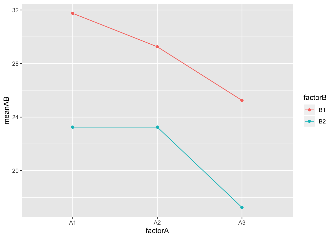
This is simply a plot of the cell means. It is important to realize that the means would still be the same if you performed a plain two-way ANOVA on this data: the only thing that changes is the error-term calculations! Notice that female students (B1) always score higher than males, and the A1 (pre) and A2 (post) are higher than A3 (control). However, in line with our results, there doesn’t appear to be an interaction (distance between the dots/lines stays pretty constant). To get all comparisons of interest, you can use the emmeans package. Notice that emmeans corrects for multiple comparisons (Tukey adjustment) right out of the box.
emmeans(fit,pairwise~factorA)## $emmeans
## factorA emmean SE df lower.CL upper.CL
## A1 27.5 1.28 11.1 24.7 30.3
## A2 26.2 1.28 11.1 23.4 29.1
## A3 21.2 1.28 11.1 18.4 24.1
##
## Results are averaged over the levels of: factorB
## Degrees-of-freedom method: kenward-roger
## Confidence level used: 0.95
##
## $contrasts
## contrast estimate SE df t.ratio p.value
## A1 - A2 1.25 1.21 12 1.035 0.5700
## A1 - A3 6.25 1.21 12 5.175 0.0006
## A2 - A3 5.00 1.21 12 4.140 0.0036
##
## Results are averaged over the levels of: factorB
## Degrees-of-freedom method: kenward-roger
## P value adjustment: tukey method for comparing a family of 3 estimatesemmeans(fit,pairwise~factorB)## $emmeans
## factorB emmean SE df lower.CL upper.CL
## B1 28.8 1.52 6 25.0 32.5
## B2 21.2 1.52 6 17.5 25.0
##
## Results are averaged over the levels of: factorA
## Degrees-of-freedom method: kenward-roger
## Confidence level used: 0.95
##
## $contrasts
## contrast estimate SE df t.ratio p.value
## B1 - B2 7.5 2.15 6 3.487 0.0130
##
## Results are averaged over the levels of: factorA
## Degrees-of-freedom method: kenward-rogerWhat about that sphericity assumption?
library(car)

#use the wide data from before to build a model

wide<-data%>%select(factorA, factorB, subj, Y)%>%spread(factorA, Y)

model<-lm(cbind(A1,A2,A3)~factorB, data=wide)

#define the within-subjects factor
A<-factor(c("A1","A2","A3"))

aov1<-Anova(model,idata=data.frame(A),idesign=~A)
summary(aov1, multivariate=F)
##
## Univariate Type II Repeated-Measures ANOVA Assuming Sphericity
##
## Sum Sq num Df Error SS den Df F value Pr(>F)
## (Intercept) 15000.0 1 166.5 6 540.540 4.152e-07 ***
## factorB 337.5 1 166.5 6 12.162 0.013024 *
## A 175.0 2 70.0 12 15.000 0.000544 ***
## factorB:A 7.0 2 70.0 12 0.600 0.564474
## ---
## Signif. codes: 0 '***' 0.001 '**' 0.01 '*' 0.05 '.' 0.1 ' ' 1
##
##
## Mauchly Tests for Sphericity
##
## Test statistic p-value
## A 0.54857 0.22289
## factorB:A 0.54857 0.22289
##
##
## Greenhouse-Geisser and Huynh-Feldt Corrections
## for Departure from Sphericity
##
## GG eps Pr(>F[GG])
## A 0.68898 0.002914 **
## factorB:A 0.68898 0.512014
## ---
## Signif. codes: 0 '***' 0.001 '**' 0.01 '*' 0.05 '.' 0.1 ' ' 1
##
## HF eps Pr(>F[HF])
## A 0.8270869 0.001377537
## factorB:A 0.8270869 0.537565255Looks reasonably well met!
Two within-subjects factors
OK, so we have looked at a repeated measures ANOVA with one within-subjects variable, and then a two-way repeated measures ANOVA (one between, one within a.k.a split-plot). Let’s look at another two-way, but this time let’s consider the case where you have two within-subjects variables. I am going to have to add more data to make this work. What I will do is, I will duplicate the control group exactly so that now there are four levels of factor A (for a total of \(4\times 8=32\) test scores).
###### Two within!

##added a second observation on all eight subjects to make a fully factored design

subj<-rep(c("S1","S2","S3","S4","S5","S6","S7","S8"),4)
factorA<-rep(c("A1","A2"),each=16)
factorB<-rep(rep(c("B1","B2"),each=8),2)
Y<-c(31,33,28,35,27,22,20,24,
     30,28,28,31,25,23,20,25,
     29,20,19,33,20,18,14,17,
     17,14,18,20,33,19,20,29)
     #29,20,19,33,20,18,14,17)

data<-data.frame(factorA, factorB, subj, Y)

data%>%arrange(subj)
## factorA factorB subj Y
## 1 A1 B1 S1 31
## 2 A1 B2 S1 30
## 3 A2 B1 S1 29
## 4 A2 B2 S1 17
## 5 A1 B1 S2 33
## 6 A1 B2 S2 28
## 7 A2 B1 S2 20
## 8 A2 B2 S2 14
## 9 A1 B1 S3 28
## 10 A1 B2 S3 28
## 11 A2 B1 S3 19
## 12 A2 B2 S3 18
## 13 A1 B1 S4 35
## 14 A1 B2 S4 31
## 15 A2 B1 S4 33
## 16 A2 B2 S4 20
## 17 A1 B1 S5 27
## 18 A1 B2 S5 25
## 19 A2 B1 S5 20
## 20 A2 B2 S5 33
## 21 A1 B1 S6 22
## 22 A1 B2 S6 23
## 23 A2 B1 S6 18
## 24 A2 B2 S6 19
## 25 A1 B1 S7 20
## 26 A1 B2 S7 20
## 27 A2 B1 S7 14
## 28 A2 B2 S7 20
## 29 A1 B1 S8 24
## 30 A1 B2 S8 25
## 31 A2 B1 S8 17
## 32 A2 B2 S8 29Notice that each subject gives a response (i.e., takes a test) in each combination of factor A and B (i.e., A1B1, A1B2, A2B1, A2B2). This is a fully crossed within-subjects design. We can see by looking at tables that each subject gives a response in each condition (i.e., there are no between-subjects factors).
table(data$factorA,data$subj)##
## S1 S2 S3 S4 S5 S6 S7 S8
## A1 2 2 2 2 2 2 2 2
## A2 2 2 2 2 2 2 2 2table(data$factorB,data$subj)##
## S1 S2 S3 S4 S5 S6 S7 S8
## B1 2 2 2 2 2 2 2 2
## B2 2 2 2 2 2 2 2 2table(data$factorA,data$factorB)##
## B1 B2
## A1 8 8
## A2 8 8Now, before we had to partition the between-subjects SS into a part owing to the between-subjects factor and then a part within the between-subjects factor. But we do not have any between-subjects factors, so things are a bit more straightforward.
However, we do have an interaction between two within-subjects factors. Indeed, you will see that what we really have is a three-way ANOVA (factor A \(\times\) factor B \(\times\) subject)!
The sums of squares for factors A and B (SSA and SSB) are calculated as in a regular two-way ANOVA (e.g., \(BN_B\sum(\bar Y_{\bullet j \bullet}-\bar Y_{\bullet \bullet \bullet})^2\) and \(AN_A\sum(\bar Y_{\bullet \bullet i}-\bar Y_{\bullet \bullet \bullet})^2\)), where A and B are the number of levels of factors A and B, and \(N_A\) and \(N_B\) are the number of subjects in each level of A and B, respectively.
Since each subject multiple measures for factor A, we can calculate an error SS for factors by figuring out how much noise there is left over for subject \(i\) in factor level \(j\) after taking into account their average score \(Y_{i\bullet \bullet}\) and the average score in level \(j\) of factor A, \(Y_{\bullet j \bullet}\). To do this, we need to calculate the average score for person \(i\) in condition \(j\), \(\bar Y_{ij\bullet}\) (we will call it meanAsubj in R)
First, let’s get our means.
data<-data%>%mutate(grand_mean=mean(Y))%>%
  group_by(factorA,factorB)%>%mutate(meanAB=mean(Y))%>%ungroup()%>%
  group_by(factorA,subj)%>%mutate(meanAsubj=mean(Y))%>%ungroup()%>%
  group_by(factorB,subj)%>%mutate(meanBsubj=mean(Y))%>%ungroup()%>%
  group_by(factorA)%>%mutate(meanA=mean(Y))%>%ungroup()%>%
  group_by(factorB)%>%mutate(meanB=mean(Y))%>%ungroup()%>%
  group_by(subj)%>%mutate(subj_mean=mean(Y))%>%
  ungroup()

data%>%arrange(subj)
## # A tibble: 32 x 11
## factorA factorB subj Y grand_mean meanAB meanAsubj meanBsubj meanA
## <fct> <fct> <fct> <dbl> <dbl> <dbl> <dbl> <dbl> <dbl>
## 1 A1 B1 S1 31 24.1 27.5 30.5 30 26.9
## 2 A1 B2 S1 30 24.1 26.2 30.5 23.5 26.9
## 3 A2 B1 S1 29 24.1 21.2 23 30 21.2
## 4 A2 B2 S1 17 24.1 21.2 23 23.5 21.2
## 5 A1 B1 S2 33 24.1 27.5 30.5 26.5 26.9
## 6 A1 B2 S2 28 24.1 26.2 30.5 21 26.9
## 7 A2 B1 S2 20 24.1 21.2 17 26.5 21.2
## 8 A2 B2 S2 14 24.1 21.2 17 21 21.2
## 9 A1 B1 S3 28 24.1 27.5 28 23.5 26.9
## 10 A1 B2 S3 28 24.1 26.2 28 23 26.9
## # … with 22 more rows, and 2 more variables: meanB <dbl>, subj_mean <dbl>Here are the data in an easier form
data%>%mutate(cellAB=interaction(factorA,factorB))%>%select(cellAB,Y,subj)%>%spread(cellAB,Y)%>%rowwise()%>%mutate(subj_mean=mean(c(A1.B1,A2.B1,A1.B2,A2.B2)))## Source: local data frame [8 x 6]
## Groups: <by row>
##
## # A tibble: 8 x 6
## subj A1.B1 A2.B1 A1.B2 A2.B2 subj_mean
## <fct> <dbl> <dbl> <dbl> <dbl> <dbl>
## 1 S1 31 29 30 17 26.8
## 2 S2 33 20 28 14 23.8
## 3 S3 28 19 28 18 23.2
## 4 S4 35 33 31 20 29.8
## 5 S5 27 20 25 33 26.2
## 6 S6 22 18 23 19 20.5
## 7 S7 20 14 20 20 18.5
## 8 S8 24 17 25 29 23.8This shows each subject’s score in each of the four conditions.
Here is the average score in each condition, and the average score for each subject
data%>%select(factorA,factorB,meanAB)%>%unique()%>%spread(factorA,meanAB)## # A tibble: 2 x 3
## factorB A1 A2
## <fct> <dbl> <dbl>
## 1 B1 27.5 21.2
## 2 B2 26.2 21.2Here is the average score for each subject in each level of condition B (i.e., collapsing over condition A)
data%>%filter(factorA=="A1")%>%select(subj,factorB,meanAsubj)%>%spread(factorB,meanAsubj)## # A tibble: 8 x 3
## subj B1 B2
## <fct> <dbl> <dbl>
## 1 S1 30.5 30.5
## 2 S2 30.5 30.5
## 3 S3 28 28
## 4 S4 33 33
## 5 S5 26 26
## 6 S6 22.5 22.5
## 7 S7 20 20
## 8 S8 24.5 24.5And here is the average score for each level of condition A (i.e., collapsing over condition B)
data%>%filter(factorB=="B1")%>%select(subj,factorA,meanBsubj)%>%spread(factorA,meanBsubj)## # A tibble: 8 x 3
## subj A1 A2
## <fct> <dbl> <dbl>
## 1 S1 30 30
## 2 S2 26.5 26.5
## 3 S3 23.5 23.5
## 4 S4 34 34
## 5 S5 23.5 23.5
## 6 S6 20 20
## 7 S7 17 17
## 8 S8 20.5 20.5Now how far is person \(i\)’s average score in level \(j\) from what we would predict based on the person-effect (\(\bar Y_{i\bullet \bullet}\)) and the factor A effect (\(\bar Y_{\bullet j \bullet}\)) alone? Just like the interaction SS above,
\[ \begin{aligned} SS_{ASubj}&={n_A}\sum_i\sum_j\sum_k(\text{mean of } Subj_i\text{ in }A_j - \text{(grand mean + effect of }A_j + \text{effect of }Subj_i))^2 \\ &={n_A}\sum\sum\sum(\bar Y_{ij\bullet} - (\bar Y_{\bullet \bullet \bullet} + (\bar Y_{\bullet j \bullet} - \bar Y_{\bullet \bullet \bullet}) + (\bar Y_{i\bullet \bullet}-\bar Y_{\bullet \bullet \bullet}) ))^2 \\ &={n_A}\sum\sum\sum(\bar Y_{ij \bullet} - (\bar Y_{\bullet j \bullet} + \bar Y_{i\bullet \bullet} - \bar Y_{\bullet \bullet \bullet}) ))^2 \\ &={n_A}\sum\sum\sum(\bar Y_{ij \bullet} - \bar Y_{\bullet j \bullet} - \bar Y_{i \bullet \bullet} + \bar Y_{\bullet \bullet \bullet} ))^2 \\ \end{aligned} \]
Where \({n_A}\) is the number of observations/responses/scores per person in each level of factor A (assuming they are equal for simplicity; this will only be the case in a fully-crossed design like this).
For example, the average test score for subject S1 in condition A1 is \(\bar Y_{11\bullet}=30.5\). The effect of condition A1 is \(\bar Y_{\bullet 1 \bullet} - \bar Y_{\bullet \bullet \bullet}=26.875-24.0625=2.8125\), and the effect of subject S1 (i.e., the difference between their average test score and the mean) is \(\bar Y_{1\bullet \bullet} - \bar Y_{\bullet \bullet \bullet}=26.75-24.0625=2.6875\). So we would expect person S1 in condition A1 to have an average score of \(\text{grand mean + effect of }A_j + \text{effect of }Subj_i=24.0625+2.8125+2.6875=29.5625\), but they actually have an average score of \((31+30)/2=30.5\), leaving a difference of \(0.9375\). Just square it, move on to the next person, repeat the computation, and sum them all up when you are done (and multiply by \(N_{nA}=2\) since each person has two observations for each level).
Since it is a within-subjects factor too, you do the exact same process for the SS of factor B, where \(N_nB\) is the number of observations per person for each level of B (again, 2):
\[ \begin{aligned} SS_{BSubj}&={n_B}\sum_i\sum_j\sum_k(\text{mean of } Subj_i\text{ in }B_k - \text{(grand mean + effect of }B_k + \text{effect of }Subj_i))^2 \\ &={n_B}\sum\sum\sum(\bar Y_{i\bullet k} - (\bar Y_{\bullet \bullet \bullet} + (\bar Y_{\bullet \bullet k} - \bar Y_{\bullet \bullet \bullet}) + (\bar Y_{i\bullet \bullet}-\bar Y_{\bullet \bullet \bullet}) ))^2 \\ &={n_B}\sum\sum\sum(\bar Y_{i\bullet k} - (\bar Y_{\bullet \bullet k} + \bar Y_{i\bullet \bullet} - \bar Y_{\bullet \bullet \bullet}) ))^2 \\ &={n_B}\sum\sum\sum(\bar Y_{i\bullet k} - \bar Y_{\bullet \bullet k} - \bar Y_{i \bullet \bullet} + \bar Y_{\bullet \bullet \bullet} ))^2 \\ \end{aligned} \]
Finally the interaction error term. This is the last (and longest) formula. Basically, it sums up the squared deviations of each test score \(Y_{ijk}\) from what we would predict based on the mean score of person \(i\) in level \(j\) of A and level \(k\) of B.
$$ \[\begin{aligned} SS_{ABsubj}&=\sum_i\sum_j\sum_k(\text{score for } Subj_i\text{ in }A_j, B_k - \text{(grand mean + effect of }A_j + \text{effect of }B_k + \text{effect of }Subj_i+\text{effect of }AB_{jk}+\text{effect of }SB_{ik} +\text{effect of }SA_{ij}))^2 \\ &=\sum\sum\sum(Y - (\bar Y_{\bullet \bullet \bullet} + (\bar Y_{\bullet j \bullet} - \bar Y_{\bullet \bullet \bullet}) + (\bar Y_{i\bullet \bullet}-\bar Y_{\bullet \bullet \bullet})+ (\bar Y_{\bullet \bullet k}-\bar Y_{\bullet \bullet \bullet}) +[\bar Y_{\bullet jk}-(\bar Y_{\bullet \bullet \bullet} + (\bar Y_{\bullet j \bullet}-\bar Y_{\bullet \bullet \bullet})+(\bar Y_{\bullet \bullet k}-\bar Y_{\bullet \bullet \bullet}))]\\ &+[\bar Y_{ ij\bullet}-(\bar Y_{\bullet \bullet \bullet} + ( \bar Y_{i \bullet \bullet}-\bar Y_{\bullet \bullet \bullet})+(\bar Y_{\bullet j \bullet}-\bar Y_{\bullet \bullet \bullet}))]+ [\bar Y_{i\bullet k}-(\bar Y_{\bullet \bullet \bullet} + (\bar Y_{i \bullet \bullet}-\bar Y_{\bullet \bullet \bullet})+(\bar Y_{\bullet \bullet k}-\bar Y_{\bullet \bullet \bullet}))]^2\\ &=\sum\sum\sum(Y - (\bar Y_{\bullet \bullet \bullet} + \bar Y_{\bullet j \bullet} - \bar Y_{\bullet \bullet \bullet} + \bar Y_{i\bullet \bullet}-\bar Y_{\bullet \bullet \bullet}+ \bar Y_{\bullet \bullet k}-\bar Y_{\bullet \bullet \bullet} +[\bar Y_{\bullet jk}- \bar Y_{\bullet j \bullet}-\bar Y_{\bullet \bullet k}+\bar Y_{\bullet \bullet \bullet}] \\&+[\bar Y_{ ij\bullet}-\bar Y_{i \bullet \bullet}-\bar Y_{\bullet j \bullet}+\bar Y_{\bullet \bullet \bullet}]+ [\bar Y_{ i\bullet k} -\bar Y_{i \bullet \bullet}- \bar Y_{\bullet \bullet k}+\bar Y_{\bullet \bullet \bullet}] )^2\\ &=\sum\sum\sum(Y -(\bar Y_{\bullet \bullet \bullet} - \bar Y_{\bullet j \bullet}- \bar Y_{i \bullet \bullet}-\bar Y_{\bullet \bullet k}+\bar Y_{\bullet jk}+\bar Y_{ij \bullet}+\bar Y_{i\bullet k}))^2\\ &=\sum\sum\sum(Y -\bar Y_{\bullet \bullet \bullet} + \bar Y_{\bullet j \bullet}+ \bar Y_{i \bullet \bullet}+\bar Y_{\bullet \bullet k}-\bar Y_{\bullet jk}-\bar Y_{ij \bullet}-\bar Y_{i\bullet k}))^2 \end{aligned}\]$$ Let’s have R calculate the sums of squares for us:
data%>%summarize(SST=sum((Y-grand_mean)^2),
                 SSA=sum((meanA-grand_mean)^2),
                 SSB=sum((meanB-grand_mean)^2),
                 SSbs=sum((subj_mean-grand_mean)^2),
                 SSAB=sum((meanAB+grand_mean-meanA-meanB)^2),
                 SSAsubj=sum((meanAsubj+grand_mean-subj_mean-meanA)^2),
                 SSBsubj=sum((meanBsubj+grand_mean-subj_mean-meanB)^2),
                 SSABsubj=sum((Y-grand_mean+meanA+meanB+subj_mean-meanAB-meanAsubj-meanBsubj)^2))
## # A tibble: 1 x 8
## SST SSA SSB SSbs SSAB SSAsubj SSBsubj SSABsubj
## <dbl> <dbl> <dbl> <dbl> <dbl> <dbl> <dbl> <dbl>
## 1 1128. 253. 3.12 355. 3.12 145. 224. 143.As before, we have three F tests: factor A, factor B, and the interaction. Each has its own error term. The degrees of freedom and very easy: \(DF_A=(A-1)=2-1=1\), \(DF_B=(B-1)=2-1=1\), \(DF_{ASubj}=(A-1)(N-1)=(2-1)(8-1)=7\), \(DF_{ASubj}=(A-1)(N-1)=(2-1)(8-1)=7\), \(DF_{BSubj}=(B-1)(N-1)=(2-1)(8-1)=7\), \(DF_{ABSubj}=(A-1)(B-1)(N-1)=(2-1)(2-1)(8-1)=7\).
To test the effect of factor A, we use the following test statistic: \(F=\frac{SS_A/DF_A}{SS_{Asubj}/DF_{Asubj}}=\frac{253/1}{145.375/7}=12.1823\), very large! We reject the null hypothesis of no effect of factor A
#pvalue
pf(12.1823, df1 = 1, df2 = 7, lower.tail = F)
## [1] 0.01012435To test the effect of factor B, we use the following test statistic: \(F=\frac{SS_B/DF_B}{SS_{Bsubj}/DF_{Bsubj}}=\frac{3.125/1}{224.375/7}=.0975\), very small. We fail to reject the null hypothesis of no effect of factor B and conclude it doesn’t affect test scores.
#pvalue
pf(.0975, df1 = 1, df2 = 7, lower.tail = F)
## [1] 0.7639465Finally, to test the interaction, we use the following test statistic: \(F=\frac{SS_{AB}/DF_{AB}}{SS_{ABsubj}/DF_{ABsubj}}=\frac{3.15/1}{143.375/7}=.1538\), also quite small. We fail to reject the null hypothesis of no interaction.
#pvalue
pf(.1538, df1 = 1, df2 = 7, lower.tail = F)
## [1] 0.7065967We can confirm our calculations using R
summary(aov(Y ~ factorA*factorB + Error(subj/(factorA*factorB)), data=data))##
## Error: subj
## Df Sum Sq Mean Sq F value Pr(>F)
## Residuals 7 355.4 50.77
##
## Error: subj:factorA
## Df Sum Sq Mean Sq F value Pr(>F)
## factorA 1 253.1 253.12 12.19 0.0101 *
## Residuals 7 145.4 20.77
## ---
## Signif. codes: 0 '***' 0.001 '**' 0.01 '*' 0.05 '.' 0.1 ' ' 1
##
## Error: subj:factorB
## Df Sum Sq Mean Sq F value Pr(>F)
## factorB 1 3.12 3.12 0.097 0.764
## Residuals 7 224.37 32.05
##
## Error: subj:factorA:factorB
## Df Sum Sq Mean Sq F value Pr(>F)
## factorA:factorB 1 3.12 3.125 0.153 0.708
## Residuals 7 143.38 20.482Looks good! How about the post hoc tests? Well, we don’t need them: factor A is significant, and it only has two levels so we automatically know that they are different! The ANOVA output on the mixed model matches reasonably well.
fit<-lmer(Y~factorA*factorB+(1|subj)+(1|subj:factorA)+(1|subj:factorB),data=data)
summary(fit)
## Linear mixed model fit by REML ['lmerMod']
## Formula: Y ~ factorA * factorB + (1 | subj) + (1 | subj:factorA) + (1 |
## subj:factorB)
## Data: data
##
## REML criterion at convergence: 181.9
##
## Scaled residuals:
## Min 1Q Median 3Q Max
## -1.3542 -0.6345 -0.2485 0.5965 2.0542
##
## Random effects:
## Groups Name Variance Std.Dev.
## subj:factorB (Intercept) 5.7900 2.4062
## subj:factorA (Intercept) 0.1444 0.3801
## subj (Intercept) 4.6039 2.1457
## Residual 20.4795 4.5254
## Number of obs: 32, groups: subj:factorB, 16; subj:factorA, 16; subj, 8
##
## Fixed effects:
## Estimate Std. Error t value
## (Intercept) 27.500 1.969 13.966
## factorAA2 -6.250 2.271 -2.752
## factorBB2 -1.250 2.563 -0.488
## factorAA2:factorBB2 1.250 3.200 0.391
##
## Correlation of Fixed Effects:
## (Intr) fctAA2 fctBB2
## factorAA2 -0.577
## factorBB2 -0.651 0.440
## fctrAA2:BB2 0.406 -0.705 -0.624anova(fit)## Analysis of Variance Table
## Df Sum Sq Mean Sq F value
## factorA 1 249.604 249.604 12.1880
## factorB 1 1.996 1.996 0.0975
## factorA:factorB 1 3.125 3.125 0.1526What about that sphericity assumption? We could try, but since there are only two levels of each variable, that just results in one variance-of-differences for each variable (so there is nothing to compare)!
library(car)

#new data, so put it in wide format
wide<-data%>%select(factorA, factorB, subj, Y)%>%transmute(cross=interaction(factorA,factorB), Y=Y, subj=subj)%>%spread(cross, Y)

model<-lm(cbind(A1.B1,A1.B2,A2.B1,A2.B2)~1,data=wide)

#define the within-subjects factors
factors<-expand.grid(factorB=c("B1","B2"),factorA=c("A1","A2"))

aov1<-Anova(model,idata=factors,idesign=~factorA*factorB)
summary(aov1,multivariate=F)
##
## Univariate Type III Repeated-Measures ANOVA Assuming Sphericity
##
## Sum Sq num Df Error SS den Df F value Pr(>F)
## (Intercept) 18528.1 1 355.37 7 364.9578 2.681e-07 ***
## factorA 253.1 1 145.38 7 12.1883 0.01011 *
## factorB 3.1 1 224.37 7 0.0975 0.76395
## factorA:factorB 3.1 1 143.38 7 0.1526 0.70770
## ---
## Signif. codes: 0 '***' 0.001 '**' 0.01 '*' 0.05 '.' 0.1 ' ' 1Real Example
A former student conducted some research for my course that lended itself to a repeated-measures ANOVA design. She had 67 participants rate 8 photos (everyone sees the same eight photos in the same order), 5 of which featured people without glasses and 3 of which featured people without glasses. Each participate had to rate how intelligent (1 = very unintelligent, 5 = very intelligent) the person in each photo looks. Finally, she recorded whether the participants themselves had vision correction (None, Glasses, Other). The response variable is Rating, the within-subjects variable is whether the photo is wearing glasses (PhotoGlasses), while the between-subjects variable is the person’s vision correction status (Correction). The variable PersonID gives each person a unique integer by which to identify them.
glasses<-read.csv("~/Downloads/glasses.csv")
glasses$PersonID<-as.factor(glasses$PersonID)
glasses$PhotoID<-as.factor(glasses$PhotoID)
head(glasses,15)
## PersonID Correction PhotoGlasses Rating PhotoID
## 1 1 Glasses No 4 1
## 2 1 Glasses Yes 4 2
## 3 1 Glasses No 4 3
## 4 1 Glasses No 4 4
## 5 1 Glasses No 3 5
## 6 1 Glasses Yes 4 6
## 7 1 Glasses Yes 4 7
## 8 1 Glasses No 4 8
## 9 2 Glasses No 3 1
## 10 2 Glasses Yes 3 2
## 11 2 Glasses No 3 3
## 12 2 Glasses No 3 4
## 13 2 Glasses No 3 5
## 14 2 Glasses Yes 3 6
## 15 2 Glasses Yes 3 7contrasts(glasses$Correction)<-contr.sum
contrasts(glasses$PhotoGlasses)<-contr.sum
aov1<-aov(Rating~Correction*PhotoGlasses+Error(PersonID/PhotoGlasses),data=glasses)
summary(aov1)##
## Error: PersonID
## Df Sum Sq Mean Sq F value Pr(>F)
## Correction 2 10.51 5.255 2.446 0.0947 .
## Residuals 64 137.46 2.148
## ---
## Signif. codes: 0 '***' 0.001 '**' 0.01 '*' 0.05 '.' 0.1 ' ' 1
##
## Error: PersonID:PhotoGlasses
## Df Sum Sq Mean Sq F value Pr(>F)
## PhotoGlasses 1 81.40 81.40 85.449 2.13e-13 ***
## Correction:PhotoGlasses 2 0.39 0.19 0.202 0.817
## Residuals 64 60.97 0.95
## ---
## Signif. codes: 0 '***' 0.001 '**' 0.01 '*' 0.05 '.' 0.1 ' ' 1
##
## Error: Within
## Df Sum Sq Mean Sq F value Pr(>F)
## Residuals 402 333.9 0.8305fit1<-lmer(Rating~Correction*PhotoGlasses+(1|PersonID),data=glasses)
anova(fit1,type=1)## Analysis of Variance Table
## Df Sum Sq Mean Sq F value
## Correction 2 4.146 2.073 2.4465
## PhotoGlasses 1 81.403 81.403 96.0749
## Correction:PhotoGlasses 2 0.386 0.193 0.2276Regardless of the precise approach, we find that photos with glasses are rated as more intelligent that photos without glasses (see plot below: the average of the three dots on the right is different than the average of the three dots on the left). We don’t need to do any post-hoc tests since there are just two levels.
glasses%>%group_by(Correction,PhotoGlasses)%>%summarize(Rating=mean(Rating))%>%
  ggplot(aes(PhotoGlasses,Rating,color=Correction,group=Correction))+geom_point()+geom_line()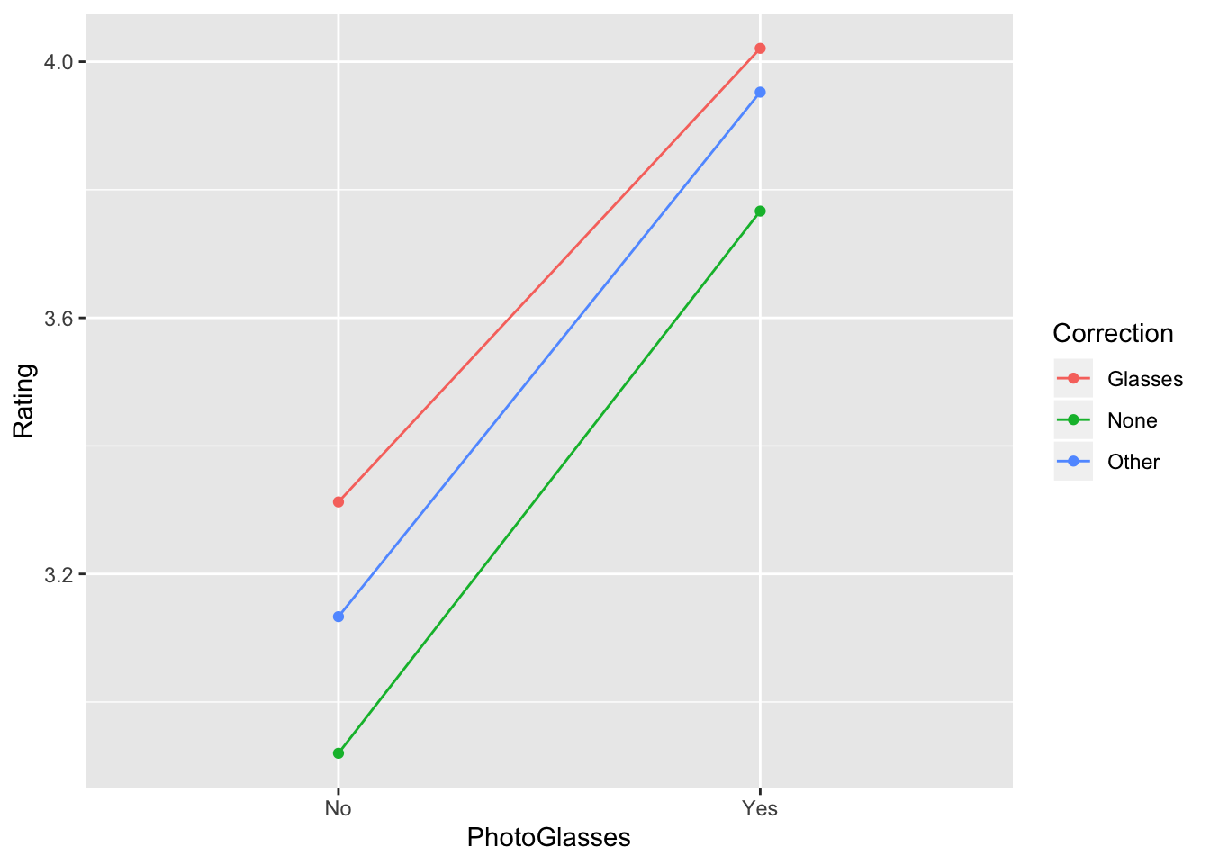
We can see that people with glasses tended to give higher ratings overall, and people with no vision correction tended to give lower ratings overall, but despite these trends there was no main effect of vision correction. There is no interaction either: the effect of PhotoGlasses is roughly the same for every Correction type.