
Modern data analysis has gotten very complicated! Let’s forget all that for a moment. I wanted to take this opportunity to examine several useful statistical techniques and measures of association that involve nothing more than a 2x2 contingency table. A 2x2 contingency table (also called a cross tabulation or cross tab) is a simple grid that displays the frequency distribution given two variables–one variable for the columnsand one variable for the rows. Suppose, for instance, that one variable is sex (male or female) and one variable is handedness (right- or left-handed). Lets say we took a random sample of 100 people and determined both their sex and their handedness. We could then take this data and create a contingency table. There are 2 possibilities for sex and 2 possibilities for handedness, resulting in 4 unique combinations: right-handed males, right-handed females, left-handed males, and left-handed females:
Here, if the proportions of individuals in different columns vary significantly between rows (or if the proportions in different rows vary between columns), we say there is a “contingency” between the two variables, and thus they are not independent of each other. This is multivariate statistics in its most basic, two-variable form, but many useful analyses arise from it. Chances are good that you’ve heard of most of them, and you may have even had occasion to use a few of them before! They are often spotted on the fringes of SPSS output but rarely ever talked about. But many can be quite useful! I’m going to talk about Chi-squared tests, Fisher-exact tests, odds ratios, and several approaches to the humble correlation coefficient (Phi, Rho, biserial, point biserial). Take a look!
Chi-Squared Test
The above table provides a framework for the examples here to come. Let’s say we give a test consisting of just 2 questions (Q1 and Q2) to a total of N students: in the table above, a is the number who got Q1 right and Q2 wrong,b is the number who got both Q1 and Q2 wrong, c is the number who got both Q1 and Q2 right, and d is the number who got Q1 wrong and Q2 right. Thus, a+b+c+d = N. Also note that a+c is the total number of students who got Q1 right, b+d is the total number who got Q1 wrong,a+b is the total getting Q2 wrong, and c+d is the total getting Q2 right. These numbers are found along the margin of the contingency table.
Now, let’s say we were interested to know whether students who got Q1 correct were more likely to get Q2 correct; that is, we want to know if scores on Q1 are correlated with scores on Q2. Let’s say we give the test to N=100 students, and here are their scores:
Start at the top rightmost cell (Q2 wrong, Q1 right). Assuming that we know only the totals, we would expect that since 49/100 (49%) of students got Q2 wrong, and since 55/100 (55%) of students got Q1 right, then 49% of 55% of the 100 students got Q2 wrong and Q1 right. Thus .49*.55*100 = **27** students. Using the totals, we can subtract 27 to calculate all of the other frequency values:
These are the frequencies we would expect to get if Q1 and Q2 were independent of each other (that is, uncorrelated). But this is not what we saw!
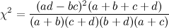
To see if these expected frequencies are significantly different from the numbers we observed, we compute a chi-squared test statistic like so:

Thus, for each cell, we subtract the expected frequency from the observed frequency, square that quantity, and divide by the expected frequency. Then we add them all up. This gives us a measure of how much our sample deviates from the expectation.

Our test statistic is 27.3; this seems big, but we need to look at a chi-squared distribution with (#rows-1)*(#cols-1) degrees of freedom. Here, that’s just 1.
Instead of going to a table of critical values, I’ll use R to make a pretty graph:
<code style="color:black;word-wrap:normal;"> > qchisq(.95,1) <br></br> [1] 3.841459 <br></br> > cord.x<-c(0, seq(0.001,3.84,.01),3.84) <br></br> > cord.y<-c(0,dchisq(seq(0.001,3.84,.01),1),0) <br></br> > curve(dchisq(x,1),xlim=c(0,10),main='Chi-Squared, df=1, a=.05') <br></br> > polygon(cord.x,cord.y,col="skyblue") <br></br></code>

If the data were independent, there is a less than 5% chance of observing a test statistic larger than 3.84; our test statistic was much larger, 27.3! Thus, it is extremely unlikely that we would observe a value that large if our data were uncorrelated. So, we reject that possibility.
Another, perhaps quicker way of computing the chi-squared test statistic is worth mentioning here.
Check out the squared quantity on top: look familiar? You’ve got a determinant here! If that quantity (ad-bc) were zero, you would know that responses to the two questions were perfectly independent. It would also be the case that the 2x2 table is “rank one” meaning that all rows are scalar multiples of the first nonzero row. To illustrate this briefly,
Multiply the top row by 2 to get the bottom row, right? Also ac-bd = 24-24=0. So here there is no association between scores on Q1 and on Q2.
But wait, back to our original example.
Measuring the extent of the relationship with correlations
Phi coefficient
Once you have your chi-squared test statistic, and you know that there is a relationship between your two categorical variables, you can easily use this number to calculate phi, which results in the same value as a correlation coefficient. If we take our chi-squared test statistic (27.3 above), divide it by the total number of people, and take the square root of that quantity, we get the phi coefficient:
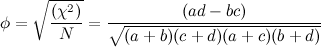
Doing this here yields $\sqrt{27.3/100}=0.522$, which is a moderate correlation. Note that this is exactly the same value as would Pearson’s r. Here’s a helpful table to help you pick the measure of association that’s right for you!
Odds Ratios
An odds ratio is another way of quantifying the size of the effect detected by chi-square significance tests of dichotomous variables. Think of the “odds” of an event as the probability of the event happening divided by the probability of it not happening. If you got Q1 right (first column), the odds of a correct answer on Q2 are (41 right)/(14 wrong), or 2.93, meaning that almost 3 times as many people got it right as got it wrong, so getting it correct is 2.93 times as likely (the odds are 2.93 to 1). We can calculate other three ‘odds’ in the same manner; of the people who got Q1 wrong (second column): 35 got Q2 right and 10 got Q2 wrong, so the odds of a right answer to Q2 given you got Q1 wrong are (10 right)/(35 wrong)=.29; thus, if you get Q1 wrong, you are more than three times as likely to get Q2 wrong than you are to get Q2 right.
Now, the odds ratio is just what it sounds like: the odds of an event happening in one group divided by the odds of it happening in another group. The ratio of two odds tells us how much more likely an event is to happen in one group versus another. Using the calculations above, we can ask, “how much more likely are the students who got Q1 right than those who got Q1 wrong to get Q2 right ?” To do this, divide the first odds of a correct Q2 of the first group (those who got Q1 right) by the odds of a correct Q2 of the second group (those who got Q1 wrong). Doing so yields $(2.93/0.29)=10.1$, which means that those who got Q1 right are 10 times more likely to get Q2 right than are those who got Q1 wrong.

If an odds ratio is greater than 1, then “A” is associated with “B” in the sense that having “A” raises the odds of having “B” (relative to not having “A”). In the present example, “Q1 Right” raises the odds of “Q2 Right” (relative to “Q1 Wrong”).
Fisher’s exact test
OK, quick aside. Imagine you have an urn containing 10 balls; 3 of them are black and 7 of them are red. If you choose 5 balls at random, what is the probability that all 5 are red? If you know a little about combinatorics, you know that there are “10 choose 5”, or 252 ways to choose 5 balls from 10:
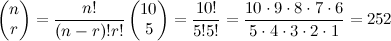
This tells us that there are 252 unique 5-ball combinations; now how many of those have 5 red balls and 0 red balls? Well, how many such combinations are there? How many ways are there to choose 5 red balls from 7 red balls? Say “7 choose 5”. Now, how many ways are there to choose 0 black balls from 3 black balls? “3 choose 0.” The product of these two combinations (7 C 5) and (3 C 0) give us the number of possible 5-ball combinations in which all 5 are red (and zero are black).
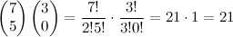
Now then, these what proportion of the total number of possible 5-ball draws (total=252) will have 5 red and 3 black (total=21)? Well,
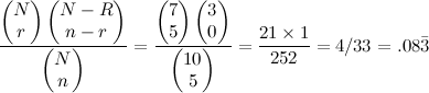
Where N is the total number of balls in the urn, R is the total number of red balls in the urn, n is the total number we select, $N-R$ is the number of black balls in the urn, r is the number of red balls in our selection, and $n-r$ is the number of black balls in our selection. Experiments of this kind follow a hypergeometric distribution, we can this method to analyze our 2x2 contingency table.
Now, instead of balls and urns, we have right and wrong. Instead of asking, “what is the probability of getting 5 red balls and 0 black balls when I draw 5 balls at random from a population that contains 7 red balls and 3 black balls” we ask “what is the probability that 14 people got Q1 right/ Q2 wrong and 35 people got Q1 wrong/ Q2 right if we draw 49 balls at random from a population where 55 got Q1 right and 45 got Q1 wrong.” That is, we want the probability of observing the given set of frequencies 14, 35, 41, 10 in a 2x2 contingency table given fixed row and column marginal totals.
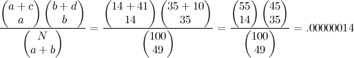
This probability is vanishingly small, but what we are really interested in is this: given our marginal frequencies, what is the chance of observing a difference at least this extreme? More extreme configurations can be generated by locating the smallest (or largest) frequency in the table, subtracting 1 (or adding 1), and then computing the remaining items given the observed marginal frequencies. When you find the collective probability of observing a combination of frequencies at least as extreme as this one, you get something smaller than $1/10,000,000$. Thus, we can conclude that answering question 1 right is associated with answering question 2 right.
Fisher’s exact test is interesting because it depends on no parametric assumptions and works for any sample size.
I may add more to this post in the future, but that’s enough for now!