
My six-year-old macbook (a black one, before the pro) is still operational, but it has burned through (literally) several batteries, and, unless I pay apple the $129.00 they want for a new one, it is going to remain about as portable as your average desktop PC. That’s fine for around-the-house applications, but when your academic adviser (who is retiring this year) asks, “Where’s your computer!” every time you have a meeting with her, you know it’s about time to get a new, backpack-friendly means of computing.
So I did! Sometime in late October I became the proud owner of a Lenovo ThinkPad T-430s (Intel i7 (3rd Gen, 2.9 GHz) processor, 16 GB of RAM and a 128 GB SSD, with an expansion bay for which I have a 500 GB HDD, an additional battery, and a DVD Multi drive) This was another high-dollar craigslist transaction (iPod, TI-89, electric guitar…) that went off without a hitch.
Anyway, it’s supposed to have this improved ThinkPad keyboard, and reviews I had read online while I was shopping around suggested that it might help to increase one’s typing speed. Around the same time, someone on Facebook posted something about play.typeracer.com, which assigns random text for you to type, calculates your WPM, and keeps a log of all the data from your past “races”. It’s great fun!
I created two accounts—one for the laptop, one for desktop (control)—and alternated playing “races” on each. I did about five on each keyboard in a sitting, over six sittings, giving me 30 games completed on each.
Subjectively, I couldn’t tell much. I seemed to be getting similar speeds regardless of which keyboard I was using.
With this data, I generated some graphs and ran two t-tests. Though “single-subject” designs are not common, I figured that it would be statistically similar to a “within-subjects” anova or a repeated-measures t-test. Given this, I figured that a sample size of ~30 per group would be sufficient.
boxplot(desktop, laptop, data=data, main="Typing Speed Data", xlab="Desktop (left) vs. Laptop (right)", ylab="Words per Minute (GPM)", col="lightblue")
Above are boxplots for the data. Notice the means appear to be roughly equal (laptop mean 84.4, desktop mean 85.2), but that there’s a lot more variation on the desktop keyboard. Below shows the scores on the desktop keyboard (blue) vs. the laptop keyboard (red) over time (should be 30 games, I typoed).
g_range<- range(70, desktop, laptop)
plot(desktop, type="o", col="blue", ylim=g_range, axes=FALSE, ann=FALSE)
axis(1, at=1:29)
axis(2, at=65:110)
box()
lines(laptop, type="o", pch=22, lty=2, col="red")
title(main="GWM over time for different keyboards")
title(xlab="Typing games played (1-29)")
title(ylab="Words per minute (WPM)")
legend(1, g_range[2], c("desktop","laptop"),cex=0.8,col=c("blue","red"),pch=21:22, lty=1:2);</blockquote>
The t-test results showed no difference between the means. My desktop scores and laptop scores are not two independent groups (because both samples were collected on one individual: me), so I used a repeated measures t-test t.test(laptop, desktop, paired=T) and got t = -0.3929, df = 29, p-value = 0.6973.
But to really know for sure, I wanted an estimate of the power of this test. Power, for those unfamiliar, is the probability of detecting differences between the groups given that there are actually differences. It is defined as one minus the probability of a type II error (failing to reject the the null hypothesis given that it is false), and can be calculated using estimates of the effect size and the sample size. A standard measure of effect size is Cohen’s d which can be calculated by the following:
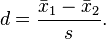 where s is equal to
 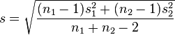 (from wikipedia)
It’s essentially a measure of the the difference between group means in terms of a pooled standard deviation. You can define function in R that will calculate this for you:
cohens_d <- function(x, y){
lx <- length(x)- 1
ly <- length(y)- 1
md <- abs(mean(x) - mean(y)) ## mean difference (numerator)
csd <- lx * var(x) + ly * var(y)
csd <- csd/(lx + ly)
csd <- sqrt(csd) ## common sd computation
cd <- md/csd ## cohen's d
}
res<-cohens_d(desktop, laptop)
res
> [1] 0.09792157
That’s a vanishingly small effect size! Power is going to be abysmal! You can calculate the power using the pwr package.
library(pwr)
pwr.t.test(30, d=.09792157, type="paired")
This yields an observed power of 0.0813, or 8% chance of detecting a difference between the groups, given that one exists! The sample size needs to be much bigger for such a small effect. To see exactly how big, I can use the pwr package again, inputting the desired power (80% is widely considered acceptable), and letting it provide me with the sample size needed.
pwr.t.test( d=.09792157, type="paired", power=.8)
n = 820!!! I would need 820 trials per keyboard for the test to be powerful enough to detect differences of that effect size. And even if we were to show that the effect was statistically significant, the effect is so small as to be not practically significant. Well, I suppose I won’t be continuing this project any time soon. I’m satisfied to know that my average WPM is 84.78 with a standard deviation of 7.77.