
One-Way ANOVA by way of Two-Sample T-Test
If the hero of our last post was William “Student” Gosset, then the hero of this and the next few posts will be Sir Ronald Fisher. After Student had derived the t distribution, he sent it to Fisher along with an historically ironic note: “I am sending you a copy of Student’s Tables as you are the only man that’s ever likely to use them!”
We have Fisher to thank for the Analysis of Variance (ANOVA), a technique which generalizes the independent two-sample t-test to more than two groups (we also have him to thank for the term “variance” itself). Echoing remarks I made in the first post of this series, ANOVA is a superb teaching/learning tool for students of inferential statistics (despite being easily subsumed by the linear model framework). There are tons of blog posts about ANOVA, but I want to walk you through the way I was taught this concept because I thought it was extremely effective.1 Let’s set the stage with a simple example first, with which we will illustate the computations required for conducting a one-way ANOVA.
Let’s say you have developed 4 different fertilizers and you want to test whether they affect plant growth differently. You have at your disposal 20 genetically identical plants, so you randomly assign each plant to one of the four fertilizer conditions. You do this because there could still be initial differences among the plants (maybe some were sprouted on the edge of the container vs the middle, etc) and randomization spreads any systematic differences out across fertilizer conditions, so that the conditions are as similar in composition as possible before they receive the treatment. Besides the fertilizer treatment, everything else about the four conditions should be held constant (amount of water, sun, etc.) so that the only variable that could plausibly account for differential plant growth is the treatment itself. Thus 5 random plants get fertilizer A, 5 get B, 5 get C, and 5 get D. After growing the plants for a fixed period of time, we collect the outcome data. Let’s measure each plant’s height in centimeters (though yield might be more appropriate). These heights are given below
| A | B | C | D |
|---|---|---|---|
| 6 | 9 | 4 | 7 |
| 7 | 10 | 6 | 9 |
| 8 | 12 | 6 | 10 |
| 9 | 14 | 6 | 11 |
| 10 | 15 | 8 | 13 |
OK then, so we want to test whether there is any difference in plant height among fertilizer groups. If we just had two groups, we could use a two-sample t-test. Considering only A and C for example (and assuming equal variances), we know that
\[ t=\frac{\bar{X}_A-\bar{X}_C}{\sqrt{s_p^2 \left(\frac{1}{n_A}+\frac{1}{n_C}\right)}} \text{ ,} \\ \begin{align} \\ s_p^2&=\frac{(n_A-1)s_A^2 + (n_B-1)s_B^2}{n_A+n_B-2}\\ \\ &= \frac{\sum_{i=1}^{n_A}(X_i-\bar{X}_A)^2 + \sum_{j=1}^{n_B}(X_j-\bar{X}_B)^2}{n_A+n_B-2}\\ \end{align} \] Since \(n_A = n_B = n\), this reduces to
\[ t=\frac{\bar{X}_A-\bar{X}_C}{\sqrt{s_p^2 \left(\frac{2}{n}\right)}} \text{ ,} \\ \begin{align} \\ s_p^2&=\frac{(s_A^2+s_B^2)}{2}\\ \\ &= \frac{\frac{\sum_{i=1}^{n}(X_i-\bar{X}_A)^2}{n-1}+\frac{\sum_{j=1}^{n}(X_j-\bar{X}_B)^2}{n-1}}{2}=\frac{\sum_{i=1}^{n}(X_i-\bar{X}_A)^2 + \sum_{j=1}^{n}(X_j-\bar{X}_B)^2}{2(n-1)}\\ \end{align} \]
Using our data for A and C, let’s calculate \(t\) using this last formula for \(s_p\) (it looks more complicated, but trust me on this).
heights<-data.frame(A=c(6,7,8,9,10), B=c(9, 10, 12, 14, 15), C=c(4,6,6,6,8), D=c(7,9,10,11,13))
n=5
meanA<-mean(heights$A); meanA
## [1] 8
meanC<-mean(heights$C); meanC
## [1] 6
# What is the difference between the mean of group A and the mean of group C?
meanDiff<-meanA-meanC; meanDiff
## [1] 2
# Now we subtract the mean of group A from each of the 5 heights in group A
deviationsA<-heights$A-meanA; deviationsA
## [1] -2 -1  0  1  2
# Same for C: we subtract the group mean from each observation in the group
deviationsC<-heights$C-meanC; deviationsC
## [1] -2  0  0  0  2
# Next, we square these differences for both groups:
sqDevsA<-deviationsA^2; sqDevsA
## [1] 4 1 0 1 4
sqDevsC<-deviationsC^2; sqDevsC
## [1] 4 0 0 0 4
# Then we add up all of these squared deviations
sumSqDevs<-sum(sqDevsA,sqDevsC); sumSqDevs
## [1] 18
# Finally, we divide by 2(n-1) to get the pooled variance
s2p<-sumSqDevs/(2*(n-1)); s2p
## [1] 2.25
Thus, our t-statistic and our test (null hypothesis: \(\mu_A = \mu_C\), alternative: \(\mu_A \ne \mu_C\)) is
tStat<-meanDiff/sqrt(s2p*(2/5))
tStat
## [1] 2.1081851-pt(tStat,8)+pt(-tStat,8)## [1] 0.06806525Thus, the probability of observing this mean difference due to chance alone is .068, and we fail to reject the null hypothesis that those two groups are different. We get the same answer by asking R to do this test for us
t.test(heights$A,heights$C,var.equal=T)##
## Two Sample t-test
##
## data: heights$A and heights$C
## t = 2.1082, df = 8, p-value = 0.06807
## alternative hypothesis: true difference in means is not equal to 0
## 95 percent confidence interval:
## -0.1876676 4.1876676
## sample estimates:
## mean of x mean of y
## 8 6We can also quickly see that our assumption of equal variances was suitable
t.test(heights$A,heights$C,var.equal = F)##
## Welch Two Sample t-test
##
## data: heights$A and heights$C
## t = 2.1082, df = 7.9024, p-value = 0.06849
## alternative hypothesis: true difference in means is not equal to 0
## 95 percent confidence interval:
## -0.1923777 4.1923777
## sample estimates:
## mean of x mean of y
## 8 6But the question still remains: how can we compare more than two groups simultaneously? Let’s say we just want an answer to the question of whether fertilizer condition affects plant height. How do we pose such a question? Specifically, how do we test the null hypothesis \(H_0: \mu_A=\mu_B=\mu_C=\mu_D\) against the alternative hypothesis that at least one of these means does not equal the others?
One-Way ANOVA
By way of a broad overview, the approach we will take to this problem is to partition the total variability into two parts: one attributable to random variability within each group/condition/treatment, and one attributable to the variability between the groups themselves. The ANOVA compares the ratio of the variability between groups to the variability within the groups—if the variability between groups is larger than the random variability within groups, then the grouping variable is said to have a significant effect on the dependent variable. Put another way, if most of the total variability (e.g., in plant height) is due to the different groups, then the grouping factor (e.g., fertilizer) is affecting the outcome more at a greater-than-chance level.
Let’s adopt some useful notation (for observations, grand mean, group means, etc) before we return to our plant-growth scenario.
For subjects (individuals, plants, students, “units”), we use the subscript \(i; \ (i=1,2,3,...,i,...,n_k)\) where \(n_k\) is the total number of observations in a given group \(k\).
For groups (conditions, treatments, etc.), we therefore use the subscript \(k; \ (k=1,2,3,...,k,...,K)\) where \(K\) is the total number of groups.
Just to be clear—because notation is super important!\(x_{ik}\) : score for subject i in group k
\(\bar{x}_{\bullet k}\) : mean of group k
\(\bar{x}_{\bullet \bullet}\): total (or “grand”) mean
| A (\(k=1\)) | B (\(k=2\)) | C (\(k=3\)) | D (\(k=4\)) | |
|---|---|---|---|---|
| \(i=1\) | \(x_{1,1}=6\) | \(x_{1,2}=9\) | \(x_{1,3}=4\) | \(x_{1,4}=7\) |
| \(i=2\) | \(x_{2,1}=7\) | \(x_{2,2}=10\) | \(x_{2,3}=6\) | \(x_{2,4}=9\) |
| \(i=3\) | \(x_{3,1}=8\) | \(x_{3,2}=12\) | \(x_{3,3}=6\) | \(x_{3,4}=10\) |
| \(i=4\) | \(x_{4,1}=9\) | \(x_{4,2}=14\) | \(x_{4,3}=6\) | \(x_{4,4}=11\) |
| \(i=5\) | \(x_{5,1}=10\) | \(x_{5,2}=15\) | \(x_{5,3}=8\) | \(x_{5,4}=13\) |
In our example data, the number of groups is \(K=4\) and the number of observations in each group is the same (\(n_1=n_2=...n_K=5\)). The total number of observations across groups is given by \(N=\sum_{k=1}^Kn_k=n_1+n_2+...n_K\)
#Sums of Squares
ANOVA works by partitioning sums of squares (actually, sums of square deviations of \(x_{ik}\) from either the group mean \(\bar{x}_{\bullet k}\) or grand mean \(\bar{x}_{\bullet \bullet}\)).
The Total Sum of Squares (\(SS_T\)) is simply the sum of the squared distance of each observation from the grand mean: \(\sum (x_{ik}-\bar{x}_{\bullet \bullet})^2\). Using our notation above, this is written \[ SS_T=\sum_{k=1}^{K}\sum_{i=1}^{n_k}(x_{ik}-\bar{x}_{\bullet \bullet})^2 \] If the double summation is uncomfortable, try reading it this way: we start with group \(k=1\) and, for all \(n_k=n_1\) subjects in group \(k=1\) we add up their squared deviations from the grand mean; then we go group \(k=2\) and do the same thing; finally, we add all of the sums of squares for the individual groups together to get the total. Thus, we can unroll the summation like so \[ SS_T=\sum_{k=1}^{K}\sum_{i=1}^{n_k}(x_{ik}-\bar{x}_{\bullet \bullet})^2=\sum_{i=1}^{n_1}(x_{i1}-\bar{x}_{\bullet \bullet})^2 + \sum_{i=1}^{n_2}(x_{i2}-\bar{x}_{\bullet \bullet})^2 + ... +\sum_{i=1}^{n_3}(x_{iK}-\bar{x}_{\bullet \bullet})^2 \] Of course, you don’t have to do it by group because addition is a commutative operation. Indeed, we could use \(N=\sum_{k=1}^Kn_k\) (the total number of subjects across all groups), we could just write the expression for SS_T like this \[ SS_T=\sum_{i=1}^{N}(x_{ik}-\bar{x}_{\bullet \bullet})^2 \] However, it will be important to think in terms of individuals within groups, so we will keep the earlier equation. The \(SS_T\) gives us the total squared deviations from the mean, and it may actually look familiar to you: in fact, it is the numerator of several variance calculations. For example, recall the the sample variance can be calculated by \[ s^2=\frac{\sum_{i=1}^n (x_i - \bar{x})^2}{n-1} \]
This should hint that we will ultimately be dealing with variances …but hold that thought! Now we begin the important business of taking our \(SS_T\) and spliting it into a component that represents random variability within each group (\(SS_W\)) and a component that represents variability between the groups themselves (\(SS_B\)). It will be important to notice immediately that \(SS_T=SS_B+SS_W\).
Let’s have a look at the Between-Groups Sum of Squares (\(SS_B\)) first
\[ SS_B=\sum_{k=1}^Kn_k\times (\bar{x}_{\bullet k}-\bar{x}_{\bullet \bullet})^2 \]
The quantity \(SS_B\) captures how far each group mean is from the grand mean. We take the difference between each group mean and the overall mean squared, times the number of individuals in group \(k\), \(n_k\), and we add these quantities up for all groups \(k=1,...,K\). If each group has the same number of observations \(n\), then this reduces to \(n\sum_{k=1}^K(\bar{x}_{\bullet k}-\bar{x}_{\bullet \bullet})^2\). Notice that if there are \(K\) groups, there will only be \(K\) deviations from the grand mean. Thus, in order to have \(N\) total terms in the sum, we weight each group mean-grand mean difference by multiplying each one by the number of subjects in its group (\(n_k\)).
For the Within-Groups Sum of Squares (\(SS_W\)), we have
\[ SS_W=\sum_{k=1}^K\sum_{i=1}^{n_k}(x_{i k}-\bar{x}_{\bullet k})^2 \]
This calculates the squared distances of each observation from its own group mean and adds these together across all groups. Notice that we have \(N\) total terms in the sum here too.
##Visualizing Sums of Squares
These formulas may be daunting at first, and it can be very helpful to see an illustration of what each one represents. So without further ado,
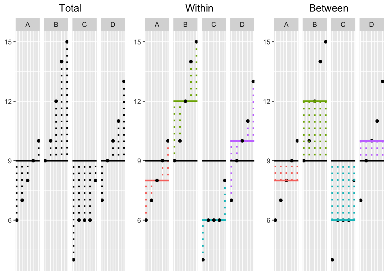
This plot is really important! It allows you to visualize the dispersion of the data in each of the three SS calculations. On the left, we have the Total deviations \((x_{ik}-\bar{x}_{\bullet \bullet})\): black dotted lines represent the deviations of each observation (large dots) from the grand mean (black bar); in the middle, we have Within-Group deviations \((x_{ik}-\bar{x}_{\bullet k})\): the deviations of each observation from their respective group mean (colored lines); on the right, we have Between-Group deviations \((x_{\bullet k}-\bar{x}_{\bullet \bullet})\): the deviations of each group mean from the grand mean times the number of observations in each group. To calculate the Total, Within-Group, and Between-Group Sums of Squares, you simply square each of the deviations in their respective plots above and then add them up, giving you three different sums.
Let’s do this and then plot our totals; here’s our data again| A | B | C | D |
|---|---|---|---|
| 6 | 9 | 4 | 7 |
| 7 | 10 | 6 | 9 |
| 8 | 12 | 6 | 10 |
| 9 | 14 | 6 | 11 |
| 10 | 15 | 8 | 13 |
| \(Mean_A\) | \(Mean_B\) | \(Mean_C\) | \(Mean_D\) |
|---|---|---|---|
| \(8\) | \(12\) | \(6\) | \(10\) |
| \(Grand \ Mean\) |
|---|
| 9 |
Calculations
Click the button to show the full sums-of-squares calculations
Sums of Squares Plot
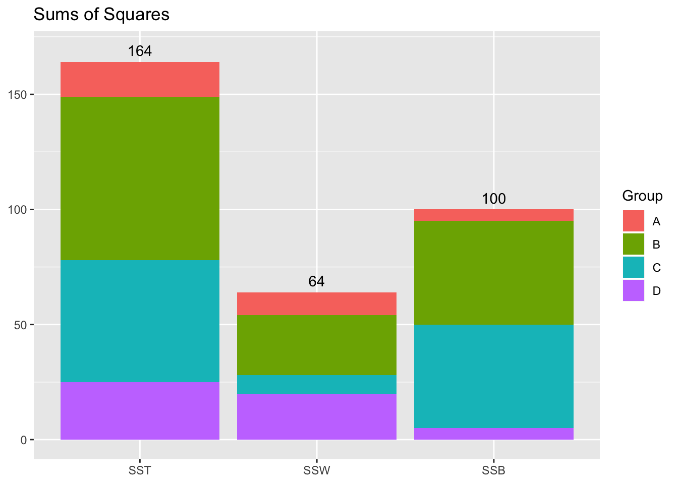
OK great, so we have our sums of squares: How do we perform the ANOVA with them? ANOVA uses an F-test for a ratio of two variances. Recall that we can think of our sums of squares as the numerator of a variance… what about the denominator? It will be helpful to consult a generic ANOVA output table:
#The ANOVA Table
| Source of Variation | SS | df | MS | F |
|---|---|---|---|---|
| Between Groups | \(SS_B=\sum_{k=1}^K n_k \times(\bar{x}_{\bullet k}-\bar{x}_{\bullet \bullet})^2\) | \(K-1\) | \(MS_B=\frac{SS_B}{K-1}\) | \(\frac{MS_B}{MS_W}\) |
| Within Groups | \(SS_W=\sum_{k=1}^K\sum_{i=1}^{n_k}(x_{i k}-\bar{x}_{\bullet k})^2\) | \(N-K\) | \(MS_W=\frac{SS_W}{N-K}\) | |
| Total | \(SS_T=\sum_{k=1}^{K}\sum_{i=1}^{n_k}(x_{ik}-\bar{x}_{\bullet \bullet})^2\) | \(N-1\) |
See those degrees of freedom (df) in the third column? You can think of those as the sample size corrected for the number of necessary interrelationships in the calculation. Remember how, when you calculate the sample variance \(\frac{\sum_i^n(x_i-\bar{x})^2}{n-1}\), you divide by n-1 instead of n? This is because in the numerator there aren’t really n independent things being added up: They are constrained by the sample mean! For example, say you want the sample variance of \(x={1,2,3}\). Well, \(\bar{x}=2\) so your \(s^2\) numerator is \((1-2)^2+(2-2)^2+(3-2)^2\), but you also know that \(3=n\bar{x}-1-2\), so you don’t even need to use 3! You can just as easly write \((1-2)^2+(2-2)^2+\left((n\bar{x}-1-2)-2\right)^2\) which becomes \((1-2)^2+(2-2)^2+\left((6-1-2)-2\right)^2\), so you don’t even need to know that \(x_3=3\).
If we consider the sums of squares calculations above, we see that the total sums of squares only has one necessary relationship among the \(N\) components: the grand mean \(\bar{X}_{\bullet \bullet}\). Thus, the denominator of this variance calculation is just like the sample variance \(N-1\). Since this isn’t a “variance” in the strict sense, we divide a sum-of-squares by its degrees-of-freedom, we refer to this quotient as the Mean Squared (MS), because it represents the “mean” of the components of the sum-of-squares.
Indeed, thought we don’t usually calculate it explicitly, the total Mean Squared is just the sample variance of the dependent variable: \(\frac{SS_T}{N-1}=\frac{164}{19}=8.6\)
var(c(heights$A,heights$B,heights$C,heights$D))## [1] 8.631579Another side note worth mentioning here: the Mean Square Within can also be found by taking the average of the group variances: \[ \begin{align} MS_W&=\frac{\sum_{k=1}^4\sum_{i=1}^{5}(x_{i k}-\bar{x}_{\bullet k})^2}{N-K} = \frac{\sum_{i=1}^{5}(x_{i k}-8)^2}{16}+\frac{\sum_{i=1}^{5}(x_{i k}-12)^2}{16}+\frac{\sum_{i=1}^{5}(x_{i k}-6)^2}{16}+\frac{\sum_{i=1}^{5}(x_{i k}-10)^2}{16}\\ \\ &= \frac{1}{4}\left(\frac{\sum_{i=1}^{5}(x_{i k}-8)^2}{4}+\frac{\sum_{i=1}^{5}(x_{i k}-12)^2}{4}+\frac{\sum_{i=1}^{5}(x_{i k}-6)^2}{4}+\frac{\sum_{i=1}^{5}(x_{i k}-10)^2}{4}\right)\\ \\ &=\frac{1}{4}\left(s^2_A+s^2_B+s^2_C+s^2_D\right)\\ \end{align} \]
mean(c(var(heights$A),var(heights$B),var(heights$C),var(heights$D)))## [1] 4##Degrees of Freedom for \(SS_W\) and \(SS_B\)
The degrees of freedom for \(SS_W\) is easy to remember too: just look at the components of the sum in the formula and note that the observations are constrained by the 4 group means, \(\bar{x}_{\bullet k}\). Thus, 20 observations go in, but once we know 4 of the observations in a given group, we automatically know the fifth one (because we have the group mean, and \(x_5=n_k\bar{x}_{\bullet k}-(x_1+x_2+x_3+x_4)\)). Thus, the degrees of freedom is given by \(N-K = 20-4 = 16\), the total number of observations minus the total number of groups.
Lastly, to find the degrees of freedom for \(SS_B\) we look at the components of the sum-of-squares calculation: here the unique observations are the group means themselves, and they are constrained by the grand mean, such that \[ n_5\bar{x}_{\bullet 5}=N\bar{x}_{\bullet \bullet}-(n_1\bar{x}_{\bullet 1}+n_2\bar{x}_{\bullet 2}+n_3\bar{x}_{\bullet 3}+n_4\bar{x}_{\bullet 4}) \] Thus, the degrees of freedom for \(SS_B\) are found by taking the number of group means and subtracting 1 for the grand mean: \(K-1=4-1=3\).
##The F-Test
We saw above that the Mean Squares are found by dividing the Sums of Squares by their DF, \(MS=\frac{SS}{df}\). Let’s fill in the ANOVA table now with all of our calculations.
| Source | SS | df | MS | F |
|---|---|---|---|---|
| Between Groups | 100 | 3 | \(\frac{SS_B}{K-1}=\frac{100}{3}\) | \(\frac{MS_B}{MS_W}=\frac{100}{12}=8.\bar{3}\) |
| Within Groups | 64 | 16 | \(\frac{SS_W}{N-K}=\frac{64}{16}\) | |
| Total | 164 | 19 |
Our F-statistic of interest is the ratio of the between-group variability (\(MS_B\)) to the within-group variability (\(MS_W\)), \(F=\frac{MS_B}{MS_W}\). (Note that any Mean Square statistic follows a chi-squared distribution, so the F-distribution gives the distribution of the ratio of two chi-squared random variables.) To see if our statistic is unusually large under the null hypothesis of no group differences (that is, to see if the between-group variance is larger than expected relative to the random within-group noise), we look at the probability of observing an F-statistic at least as large as this one under the null hypothesis. Note that the F distribution depends on two parameters: the numerator degrees of freedom (\(K-1=3\)) and the denominator degrees of freedom (\(N-K=16\)), so our test statistic follows the distribution \(F_{(3,16)}\):
F.stat<-(100/12)
numer.df<-3
denom.df<-16

x1<-seq(F.stat,10,len=100)
x2<-seq(qf(.95,numer.df,denom.df),10,len=100)
y1<-df(x1,numer.df,denom.df)
y2<-df(x2,numer.df,denom.df)
{curve(df(x,numer.df,denom.df),main="",xlim=c(0,10),xlab="F")
polygon(c(x2[1],x2,x2[100]),c(0,y2,0),col="black",border=NA)
polygon(c(x1[1],x1,x1[100]),c(0,y1,0),col="grey",border=NA)
abline(v=F.stat,lty=2)}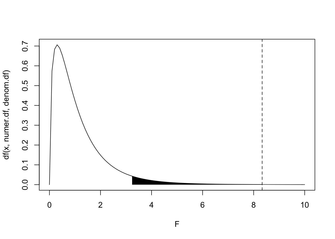
#p-value
1-pf(F.stat,numer.df,denom.df)
## [1] 0.0014506We see in the plot above that the probability of observing an F-statistic of \(8.\bar{3}\) (dotted line) or larger under the null hypothesis is very unlikely, \(p>F=.001\). The area in black under the \(F_{(3,16)}\) marks of 5% of the probability distribution. Anything observed F-statistic in the black region would reject the null hypothesis (that group means do no differ) at the traditional significance level \(\alpha=.05\). Another way of stating the null hypothesis is this: all groups are random samples of the same population, and thus that all treatments result in the same effect. Rejecting the null hypothesis means we have non-negligible evidence that different treatments result in different effects.
###Why Does This Work?
The expected value of the within-group variance is equal to the population variance, \(E(MS_W)=\sigma^2\). However, it can be shown that the expected value of the between-group variance is equal to the population variance plus an additional term representing the variabiliy of the group means around the grand mean, \(E(MS_B)=\sigma^2 + \frac{\sum_{k=1}^Kn_k (\mu_{\bullet k}-\mu_{\bullet \bullet})^2}{K-1}\). Under the null hypothesis \(\mu_1=\mu_2=...=\mu_K\), this second term will equal zero, because for all \(k\), \((\mu_{\bullet k}-\mu_{\bullet \bullet})=0\). Thus, under \(H_0\), the expected value of the F-statistic is \(E(F_{stat})=E\left(\frac{MS_B}{MS_W}\right)=\frac{\sigma^2}{\sigma^2}=1\). If our observed F-statisic is significantly larger than 1 (due to large differences between group means and thus a large \(\frac{\sum_{k=1}^Kn_k (\mu_{\bullet k}-\mu_{\bullet \bullet})^2}{K-1}\) term) than we have evidence against our null hypothesis, suggesting that at least one of the group means is different from the others.
##Doing a One-Way ANOVA in R
Performing a one-way ANOVA in R is very straightforward. Notice that R gives exactly the same results as our hand calculations. Note also that “Mean Squared Residuals” (or “Mean Squared Error”, MSE) refers to the same thing as “Mean Squared Within”—it is whatever variability is left over after accounting for the effect of the groups.
anova1<-aov(Height~Group,data=dat.long)
summary(anova1)
## Df Sum Sq Mean Sq F value Pr(>F)
## Group 3 100 33.33 8.333 0.00145 **
## Residuals 16 64 4.00
## ---
## Signif. codes: 0 '***' 0.001 '**' 0.01 '*' 0.05 '.' 0.1 ' ' 1Effect Size
Effect size is just what it sounds like: a measure of the strength of an effect or treatment. These go hand-in-hand with any hypothesis test, because a hypothesis test alone tells you nothing about the size of an effect per se, but only that it is statistically significant. For example, if you have an enormous sample size, then you have very high power to detect small differences. However, these small differences may not be practically significant, and effect sizes are crucial for giving context to any significance test.
A common effect-size measure for ANOVA is the eta-squared (\(\eta^2\)), which is the ratio of the \(SS_B\) to the \(SS_T\), \(\eta^2=\frac{SS_B}{SS_T}\). In our example above, we have \(\eta^2=\frac{100}{164}=.61\) This is a measure of the variance of the dependent variable explained by the treatment in our sample. If you are familiar with regression output, it is equivalent to the R^2.
Another common effect-size measure for ANOVA is cohen’s \(f^2\), which is calculating using \(\eta^2\), \(f^2=\frac{\eta^2}{1-\eta^2}\). We can see by looking that \(f^2\) is the ratio of variance explained to the variance not explained. Here, we would have \(.61/.39=1.56\).
According to Cohen’s (1988) guidelines (which were meant only for the social sciences, are a bit out of date, and are certainly oversimplifications), \(f^2 \ge 0.02, f^2 \ge 0.15,\) and \(f^2 \ge 0.35\) represent small, medium, and large effect sizes, respectively. According to this, the effect of our treatment is huge.
Assumptions
It is incumbent upon any user of a hypothesis-testing procedure to check the test’s underlying assumptions if they want the conclusions they draw from it to be valid. The assumptions that must be met for an ANOVA are similar to those for a t-Test, namely independent, normality (of errors), and equal variance across groups.
Independence
This one is pretty easy: a given observation should have no influence on any of the others. There are plenty of situations when this simplifying assumption doesn’t hold (imagine if you measure the same person twice!) and we will deal with these situations in the next post. For now, one plant’s height should give you no information about another plant’s height beyond knowing what fertilizer treatment they were exposed to. We achieved this by randomizing which plants got which treatment: thus, on average, the only thing different about each group should be their treatment exposure.
Normality (of Errors)
One easy way to check normality is to look at the distribution of data in each group: if these distributions are normal, then the errors (or residuals) will be normal. Fine, but what’s a residual? We will show in the next post that ANOVA is a special case of regression, in which the concept of residuals plays a crucial role. ANOVA analyses tend to gloss over residuals, but let’s take a minute to compute them.
A residual is what’s left over after we account for the effect of our independent variables. In our example, once we account for the fertilizer treatment group mean \(\bar{x}_{\bullet k}\), the residual is what’s left over. ANOVA assumes that these Within-Group deviations \((x_{ik}-\bar{x}_{\bullet k})\) are normally distributed. Here’s our data again:
| A | B | C | D |
|---|---|---|---|
| 6 | 9 | 4 | 7 |
| 7 | 10 | 6 | 9 |
| 8 | 12 | 6 | 10 |
| 9 | 14 | 6 | 11 |
| 10 | 15 | 8 | 13 |
| \(Mean_A\) | \(Mean_B\) | \(Mean_C\) | \(Mean_D\) |
|---|---|---|---|
| \(8\) | \(12\) | \(6\) | \(10\) |
So, going down columns, our residuals \((x_{ik}-\bar{x}_{\bullet k})\) are \((6-8),(7-8),(8-8),...,(10-10),(11-10),(13-10)\).
We can get these straight from our ANOVA object in R; typically, they are examined using a quantile-quantile plot (theoretical vs. observed data quantiles should be similar) or tested formally with the Shapiro-Wilk test (which tends to be overly harsh).
round(anova1$residuals,4)## 1 2 3 4 5 6 7 8 9 10 11 12 13 14 15 16 17 18 19 20
## -2 -1 0 1 2 -3 -2 0 2 3 -2 0 0 0 2 -3 -1 0 1 3{qqnorm(anova1$residuals); qqline(anova1$residuals)}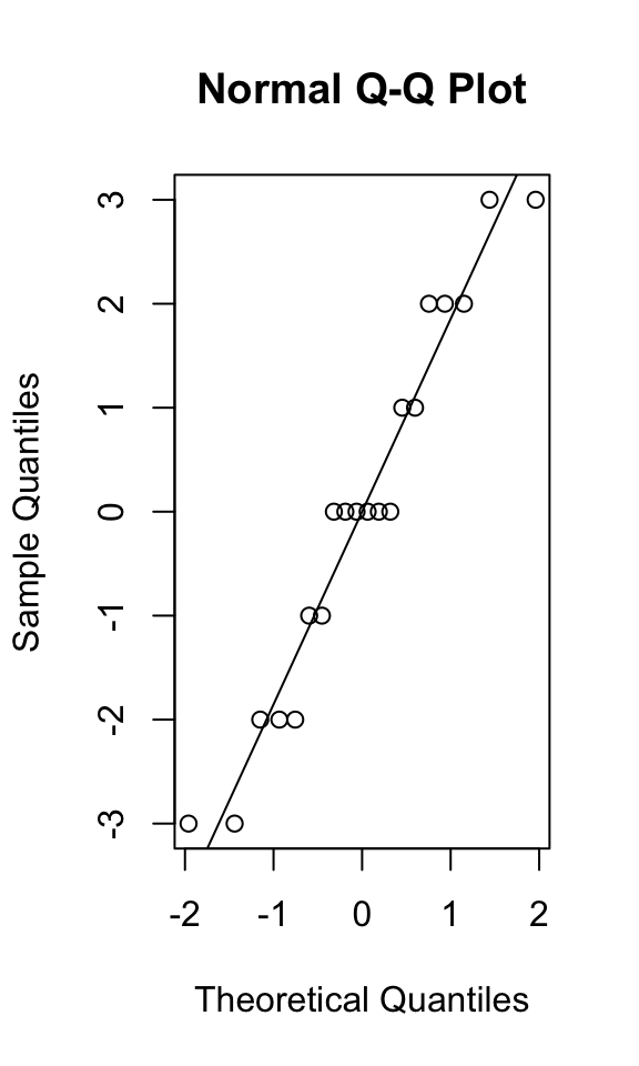
shapiro.test(anova1$residuals)##
## Shapiro-Wilk normality test
##
## data: anova1$residuals
## W = 0.94361, p-value = 0.2804In the S-W test, the null hypothesis is that the data are normally distributed: here, we fail to reject that null hypothesis, confirming what we see in our Q-Q plot (the quantiles of a normal distribution look similar to the quantiles of our observed data).
Equal Variance (Homoskedasticity)
Fortunately, ANOVA is very robust to non-normality (provided the groups are roughly symmetrical and, if skewed, skewed the same way) and relatively robust to unequal variances (provided the sample size in each group is about the same). Looking at our box plots, we see that the spreads look a little different across the four groups. However, two standard procedures for testing the null hypothesis that group variances are equal (Bartlett’s test and Levene’s test) both fail to reject this assumption.
library(car)## Loading required package: carDataboxplot(dat.long$Height~dat.long$Group)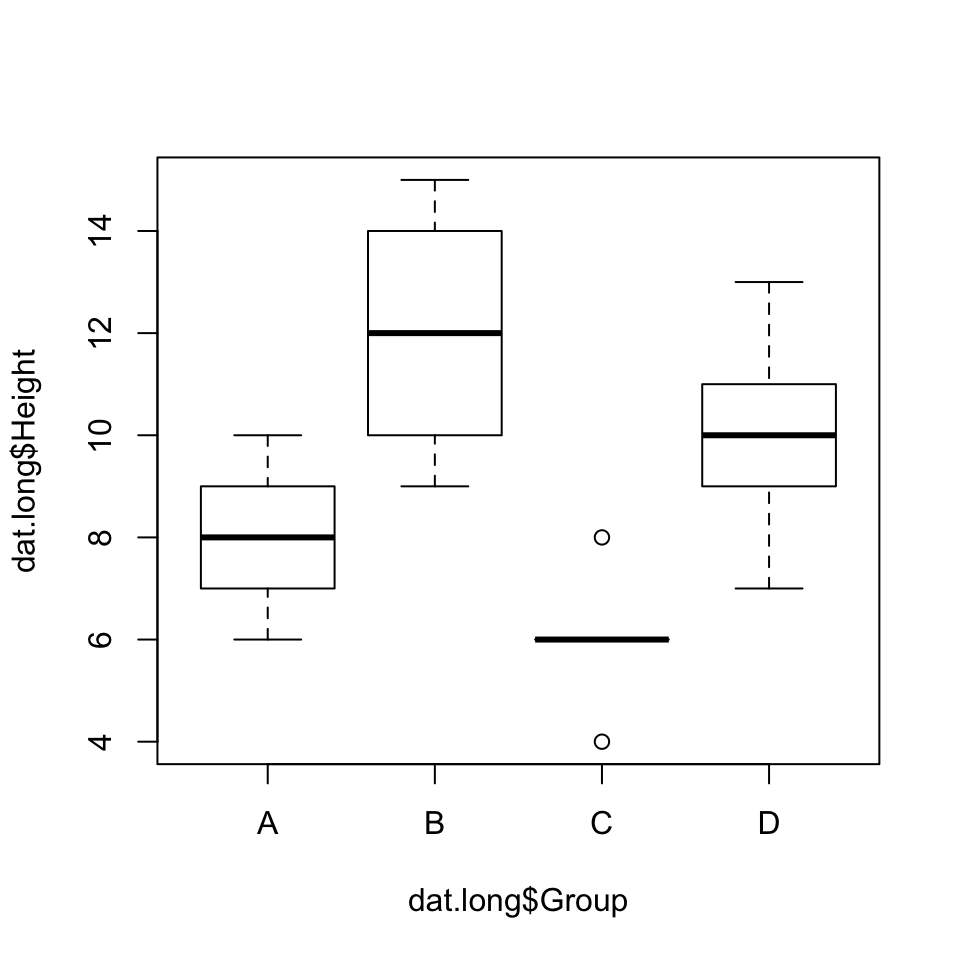
bartlett.test(dat.long$Height~dat.long$Group)##
## Bartlett test of homogeneity of variances
##
## data: dat.long$Height by dat.long$Group
## Bartlett's K-squared = 1.6465, df = 3, p-value = 0.6489leveneTest(dat.long$Height~dat.long$Group)## Levene's Test for Homogeneity of Variance (center = median)
## Df F value Pr(>F)
## group 3 1.0256 0.4075
## 16Post Hoc Tests
After performing an ANOVA which as revealed a significant effect for a factor, we know that not all groups are the same in terms of there score on the outcome variable, but we know little else. Therefore, it is often of interest to conduct a few more tests to see which groups (levels of the factor) are actually different from one another. The most common approach is to conduct t-tests between each possible pair of groups while correcting for multiple comparisons. In our example, we have 4 means (A, B, C, D), and so we have \(4 \choose{2}\) \(=\frac{4!}{2!2!}=6\) unique group comparisons \(\{AB, AC, AD, BC, BD, CD\}\). Unfortunately, the more hypotheses we test, the more likely we are to get a significant difference due to chance alone. To see this, note that when we say \(\alpha=.05\) for a given test, it means that it has a probability of 5% that a “significant” difference is due to chance alone. If we were to conduct 6 such tests (e.g., t-tests), the probability of making a Type I error (incorrectly rejecting \(H_0\)) for at least 1 of these comparisons is much greater than \(\alpha=.05\), it’s \(\alpha_{familywise}=1-(1-\alpha)^6=1-.95^6=1-.735=.265\). Thus, the probability of observing a significant difference in one of the 6 comparisons—the overall probability of making at least false rejection of H_0—is actually 26.5%! When we do multiple significance tests, we want to set the familywise (or overall) error rate at 5% instead, and there are many techniques for doing so.
###Tukey’s Test
One way around this is to use an approach variously refered to as Tukey’s test, Tukey’s HSD (honestly significant difference), Tukey’s paired comparisons, etc.
For example, to test whether Group A and Group B differed in Height, we would calculate q
\[
q=\frac{|\bar{x}_A-\bar{x}_B|}{\sqrt{MS_W/n}}=\frac{|8-14|}{\sqrt{4/5}}=2\sqrt5=4.472
\]
We look this value up in table for the studentized-range distribution to find the p-value (or probability of observing a statistic at least as extreme under the null hypothesis), which can be found in R by ptukey(q,nmeans=K,df=N-K,lower.tail=F)
ptukey(4.472,nmeans=4,df=16,lower.tail=F)## [1] 0.02779534We can easily get this for all pairwise comparisons with the TukeyHSD() function, which takes ANOVA-type model as its argument:
TukeyHSD(anova1)## Tukey multiple comparisons of means
## 95% family-wise confidence level
##
## Fit: aov(formula = Height ~ Group, data = dat.long)
##
## $Group
## diff lwr upr p adj
## B-A 4 0.3810644 7.618936 0.0277901
## C-A -2 -5.6189356 1.618936 0.4161607
## D-A 2 -1.6189356 5.618936 0.4161607
## C-B -6 -9.6189356 -2.381064 0.0011369
## D-B -2 -5.6189356 1.618936 0.4161607
## D-C 4 0.3810644 7.618936 0.0277901Thus, we see that groups A and B are significantly different, C and B are significantly different, and D and C are significantly different while holding the familywise error rate for all six comparisons at \(\alpha_{fw}=.05\), because unlike t-tests, the Tukey test applies simultaneously to all pairwise comparisons.
If you find yourself with unequal sample sizes across groups, you simply use the harmonic mean of the group sizes \(n_k\), \(\frac{K}{\sum_{k=1}^K \frac{1}{n_k}}=\frac{K}{\frac{1}{n_1}+\frac{1}{n_2}+...\frac{1}{n_K}}\), instead of \(n\) in your calculation of q.
Bonferroni T-Tests
Another approach is to say OK, we are doing 6 tests, so lets set the familywise error rate to \(\alpha_{fw}=\frac{\alpha}{5}=\frac{.05}{6}=.008\bar{3}\). Thus, for any one of our paired comparisons to be different, we would need to observe a \(p<.008\bar{3}\). This method is much more conservative (that is, it tends to over-correct, making it more likely that we make a Type II error by failing to reject a false \(H_0\)). We can see this by running all 6 t-tests like so:
# A vs. B
t.test(dat.long[dat.long$Group=='A',]$Height,dat.long[dat.long$Group=='B',]$Height,var.equal = T)$p.value
## [1] 0.01756221
#
# A vs. C
t.test(dat.long[dat.long$Group=='A',]$Height,dat.long[dat.long$Group=='C',]$Height,var.equal = T)$p.value
## [1] 0.06806525
#
# A vs. D
t.test(dat.long[dat.long$Group=='A',]$Height,dat.long[dat.long$Group=='D',]$Height,var.equal = T)$p.value
## [1] 0.1411133
#
# B vs. C
t.test(dat.long[dat.long$Group=='B',]$Height,dat.long[dat.long$Group=='C',]$Height,var.equal = T)$p.value
## [1] 0.00175135
#
# B vs. D
t.test(dat.long[dat.long$Group=='B',]$Height,dat.long[dat.long$Group=='D',]$Height,var.equal = T)$p.value
## [1] 0.2237477
#
# C vs. D
t.test(dat.long[dat.long$Group=='C',]$Height,dat.long[dat.long$Group=='D',]$Height,var.equal = T)$p.value
## [1] 0.009632847
Notice here that only B vs. C is found to be significantly different at \(\alpha=.008\bar{3}\) whereas using Tukey’s test, A vs. B and C vs. D were significant as well.
Stepdown: Bonferroni-Holm
We will look at one last correction that is a less conservative variation on bonferroni. Here, we run our six t-tests like we did above, and we sort our p-values from least to greatest:
bf_holm<-data.frame(Comparison=c("AB","AC","AD","BC","BD","CD"),Pvalue=c(
t.test(dat.long[dat.long$Group=='A',]$Height,dat.long[dat.long$Group=='B',]$Height,var.equal = T)$p.value,
t.test(dat.long[dat.long$Group=='A',]$Height,dat.long[dat.long$Group=='C',]$Height,var.equal = T)$p.value,
t.test(dat.long[dat.long$Group=='A',]$Height,dat.long[dat.long$Group=='D',]$Height,var.equal = T)$p.value,
t.test(dat.long[dat.long$Group=='B',]$Height,dat.long[dat.long$Group=='C',]$Height,var.equal = T)$p.value,
t.test(dat.long[dat.long$Group=='B',]$Height,dat.long[dat.long$Group=='D',]$Height,var.equal = T)$p.value,
t.test(dat.long[dat.long$Group=='C',]$Height,dat.long[dat.long$Group=='D',]$Height,var.equal = T)$p.value))

bf_holm[order(bf_holm$Pvalue),]
## Comparison Pvalue
## 4 BC 0.001751350
## 6 CD 0.009632847
## 1 AB 0.017562209
## 2 AC 0.068065248
## 3 AD 0.141113281
## 5 BD 0.223747695Now then, the Bonferroni-Holm procedure is as follows
- Rank comparisons from smallest p-value to largest (\(c=1,2,...N_c\))
- Start with the comparison with the smallest p-value (i.e., \(c=1\))
- Set the \(\alpha_c\) for each comparison \(c\) at \(\frac{.05}{(N_c+1)-c}\).
- If \(p_1 \le \alpha_1\), move on to \(c=2\)
- STOP when \(p_c \not\le \alpha_c\) (no more tests)
For example, our smallest p-value is \(BC\) and we have \(\alpha_1=\frac{.05}{(6+1)-1}=\frac{.05}{6}=.008\bar{3}\). So for the first comparison, the p-value is the same as Bonferroni. Since \(.00175 \le .008\bar{3}\), we say that groups \(B\) and \(C\) are significantly different, and we move on to our the comparison with the second-smallest p-value, \(CD\). Here we get \(\alpha_2=\frac{.05}{(6+1)-2}=\frac{.05}{5}=.01\), and since \(p_2=.00963<.01\), groups \(C\) and \(D\) are significantly different. For the comparison with the third-smallest p-value, \(AB\), we have \(\alpha_3=\frac{.05}{(6+1)-3}=\frac{.05}{4}=.0125\), but since \(p_3=.0176 \not\le .0125\), groups \(A\) and \(B\) are not significantly different, and we stop.
Notice that using this procedure, 2 comparisons were found to be significantly different (compared to 1 using Bonferonni and 3 using Tukey).
Also note that the Bonferonni and Bonferroni-Holm procedures and general and can be used for any set of hypothesis tests that one is conducting.
####End
I hope you have enjoyed this introduction to ANOVA! I wanted to talk about power analysis but I think I had better save this topic for the next ANOVA post, where we deal with multifactor designs like the two-way ANOVA and where we discuss interactions. Stay tuned!
####Postscript (What to do if your ANOVA assumptions are violated)
If your assumptions are violated (e.g, if your samples are too small to assess normality), you can use the non-parametric Kruskal Wallis test. It tests whether the distribution of your response variable is the same across groups: if the distributions are similar, you can interpret it as testing whether there is a difference in medians between groups.
kruskal.test(Height~Group,data=dat.long)##
## Kruskal-Wallis rank sum test
##
## data: Height by Group
## Kruskal-Wallis chi-squared = 12.291, df = 3, p-value = 0.006451Thanks Dr. Emmer, Professor Emeritus at UT Austin, In whose last-class-ever I learned so much!↩