Part 2: the t-Distribution

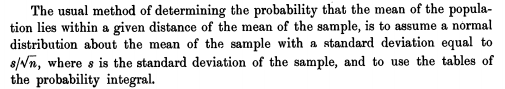
We saw in the previous post that if X is a random variable and the population distribution of X is normal with mean \(\mu\) and standard deviation \(\sigma\) (variance \(\sigma^2\)), then the distribution of the sample mean \(\bar{X}\) for samples of a given size \(n\) is normal, with mean \(\mu\) and standard deviation of \(\frac{\sigma}{\sqrt{n}}\), which we can write \(\bar{X}_n \sim N(\mu,\frac{\sigma}{\sqrt{n}})\).¹ More exciting, we saw that by the Central Limit Theorem, the sampling distribution will be normal regardless of the original population distribution if the sample size is large enough.

Recall that a Z-score is computed \(Z=\frac{\bar{X}-\mu}{\sigma/\sqrt{n}}\) If you haven’t seen this before, realize that we are just rescaling our sampling distribution from the previous post, \(\bar{X} \sim N(\mu,\frac{\sigma}{\sqrt{n}})\), in order to preserve all of the information while setting the mean to 0 and the standard deviation to 1. Another way to think of it is that, instead of dealing in terms of the sample mean \(\bar{X}\), we want to deal in terms of the distances of the sample mean from the population mean \(\bar{X}-\mu\) in units of standard deviation \(\sigma\), and we can do that by transforming \(\bar{X} \sim N(\mu,\sigma^2/n)\) into \(Z=\frac{\bar{X}-\mu}{\sigma/\sqrt{n}}\).

We can do this because a normal random variable \(X\) is still normal when it undergoes a linear transformation (multiplying it, adding to it, etc). This means that if \(X\sim N(\mu,\sigma)\), then \(Y=aX+b\) is also normal, \(Y\sim N(a\mu+b,a\sigma)\). Using this property,

\[\bar{X}-\mu \sim N(\mu-\mu,\frac{\sigma}{\sqrt{n}}) = N(0,\frac{\sigma}{\sqrt{n}})\] And

\[\frac{\bar{X}-\mu}{\sigma/\sqrt{n}} \sim N(\frac{0}{\sigma/\sqrt{n}},\frac{\sigma/\sqrt{n}}{\sigma/\sqrt{n}})= N(0,1)\].

Here’s a quick example just so you can see this in action: the heights (in inches) of adult women in the US are distributed as \(N(63.8,2.7)\). Let’s say you, \(X_1\), are a 5’8" woman (68 inches tall).

dist<-rnorm(10000,63.8,2.7)

{hist(dist,breaks=100,main="",prob=T)
curve(dnorm(x,63.8,2.7),add=T,col="blue")
abline(v=68,col="red")
text(68,.1,"68")}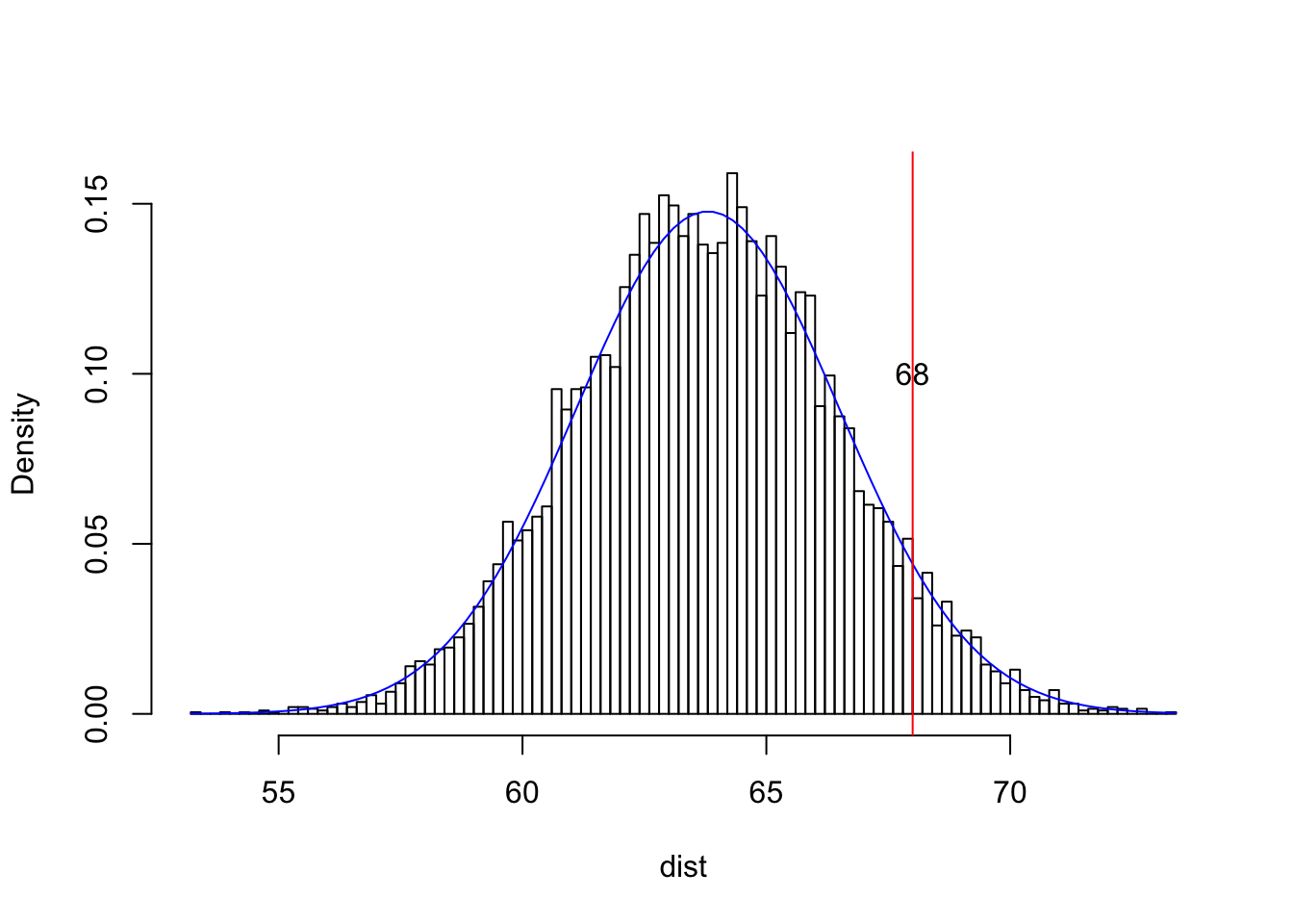

# Now we subtract the population mean from every observation in our sample

dist.minus.mean<-dist-63.8
{hist(dist.minus.mean,breaks=100,main="",prob=T)
  curve(dnorm(x+63.8,63.8,2.7),add=T,col="blue")
#notice how adding the mean y=f(x+63.8)
abline(v=68-63.8,col="red")
text(4.2,.1,"4.2")}

# See how nothing changed except the x-axis; we have effectively scooted the entire distribution right, so that it is centered at zero. Now let's divide each observation by the population standard deviation$

dist.minus.mean.dividedby.sd<-dist.minus.mean/2.7
{hist(dist.minus.mean.dividedby.sd,breaks=100,main="",prob=T)
curve(dnorm(x,0,1),add=T,col="blue")
abline(v=(68-63.8)/2.7, col="red")
text(2,.3,labels="1.555555")}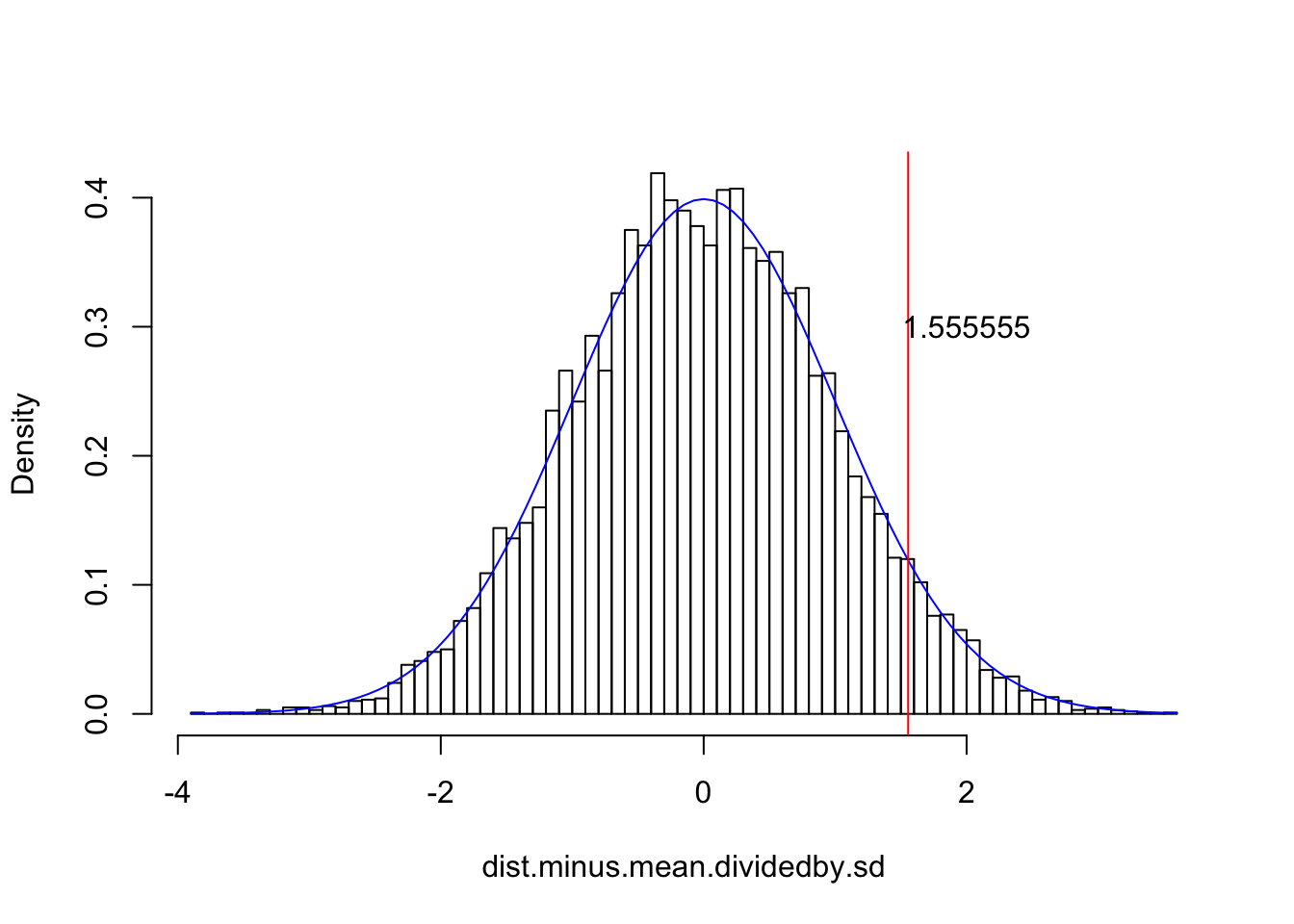

I drew a sample of 10,000 from such a distribution just to illustrate how subtracting the mean from each of those 10,000 values and then dividing each by the standard deviation preserves the normality of the sample (see distribution overlayed in blue).

Recall too that, if our statistic is normally distributed, 95% of the density should lie within 1.96 standard deviations of the mean. Here, pnorm is the CDF for the normal distribution: it gives us the area under the curve from \(-\infty\) to \(q\), where q is a Z-score.

pnorm(1.96)-pnorm(-1.96)

## [1] 0.9500042

OK, now back to STUDENT:

Here’s what he means. Let’s take repeated samples of 10 students’ heights and calculate the \(\bar{X}\) and \(s\) for each.

samps10<-matrix(nrow=10,ncol=10000)
samps10<-replicate(10000,sample(pop.height,10))
samps.mean<-apply(samps10,2,mean)
samps.sd<-apply(samps10,2,sd)

Now, is it really true that, when we substitute \(s\) for \(\sigma\) that 95% of the time the true population mean lies within \(\bar{X}\pm 1.96*s/\sqrt{n}\)?

s10.s<-mean(samps.mean-1.96*samps.sd/sqrt(10)> pop.mean | pop.mean>samps.mean+1.96*samps.sd/sqrt(10))
s10.s

## [1] 0.0854

Hmm, it looks like the population mean is actually outside this range 8.54% of the time. Clearly, when we do not know \(\sigma\), we cannot substitute \(s\) with impunity. Again, had we known \(s\), things would have been fine:

samps10<-matrix(nrow=10,ncol=10000)
samps10<-replicate(10000,sample(pop.height,10))
samps.mean<-apply(samps10,2,mean)
s10.sigma<-mean(samps.mean-1.96*pop.sd/sqrt(10)> pop.mean | pop.mean>samps.mean+1.96*pop.sd/sqrt(10))
s10.sigma

## [1] 0.0466

Using the population standard deviation, we find that the population mean falls outside two standard errors of the sample mean just 4.66% of the time. But this is no help to us in the real world!

Things just get worse with smaller samples. Here’s what happens if we just have \(n=3\)

samps3<-matrix(nrow=3,ncol=10000)
samps3<-replicate(10000,sample(pop.height,3))
samps3.mean<-apply(samps3,2,mean)
samps3.sd<-apply(samps3,2,sd)
s3.s<-mean(samps3.mean-1.96*samps3.sd/sqrt(3)> pop.mean | pop.mean>samps3.mean+1.96*samps3.sd/sqrt(3))
s3.s

## [1] 0.2059

Yikes, now the population mean falls outside our 95% confidence interval 20.59% of the time; clearly, assuming normality is inappropriate when samples are small and we are using \(s\) instead of \(\sigma\).

This problem was solved by William Sealy Gosset (“Student”") in 1908, whose paper is excerpted throughout this post

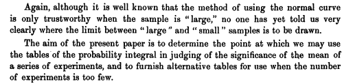
The “alternative” he furnishes is none other than the \(t\) distribution.² I will walk us through the derivations in his celebrated paper at the bottom, but as makes for an enormous, excruciating tangent, I will give a brief overview:

1. First, he determines the sampling distribution of standard deviations drawn from a normal population; he finds that this agrees with the Chi-squared distribution

2. The, he shows that there is no correlation between the sample mean and the sample standard deviation (suggesting that the two random variables are independent).

3. Finally, he determines the distribution of t (which he calls \(z\)), which is the distance between the sample mean and the population mean, divided by the sample standard deviation \(\frac{\bar{x}-\mu}{s/\sqrt{n}}\) (note the n in the denominator instead of our n-1)

First, he shows that

\[ x=\frac{(n-1)}{\sigma^2}s^2 \sim \chi^2_{n-1}, \text{ that is, it has the density}\\ p(x|n) =\frac{1}{2^{\frac{n-1}{2}}\Gamma(\frac{n-1}{2})}x^{\frac{n-1}{2}-1}e^{-\frac{x}{2}} \]

Can we confirm this? Recall that our population variance \(\sigma^2\) was 15.5544059, so let’s plot ’em and see if this density fits

#The distribution of sample variance when n=3
n=3
{hist((n-1)/(pop.sd^2)*samps3.sd^2,prob=T,breaks=50)
curve(1/(2^((n-1)/2)*gamma((n-1)/2))*x^((n-1)/2-1)*exp(-x/2),xlim=c(0,30),add=T)
curve(dchisq(x,df=2),add=T)}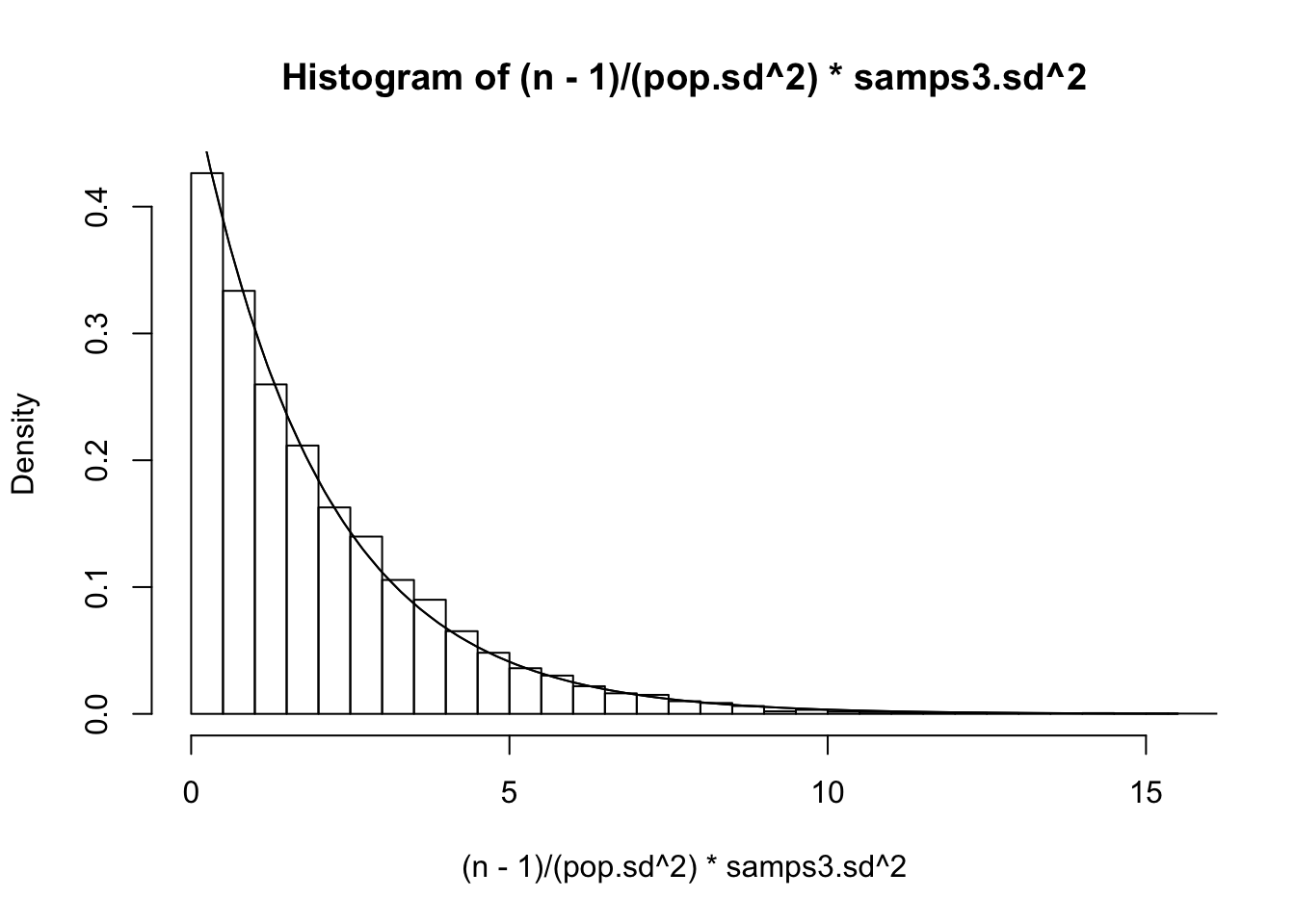

#The distribution of the sample variance when n=10
n=10
{hist((n-1)/(pop.sd^2)*samps.sd^2,prob=T,breaks=50)
curve(1/(2^((n-1)/2)*gamma((n-1)/2))*x^((n-1)/2-1)*exp(-x/2),xlim=c(0,30),add=T)
curve(dchisq(x,df=9),add=T)}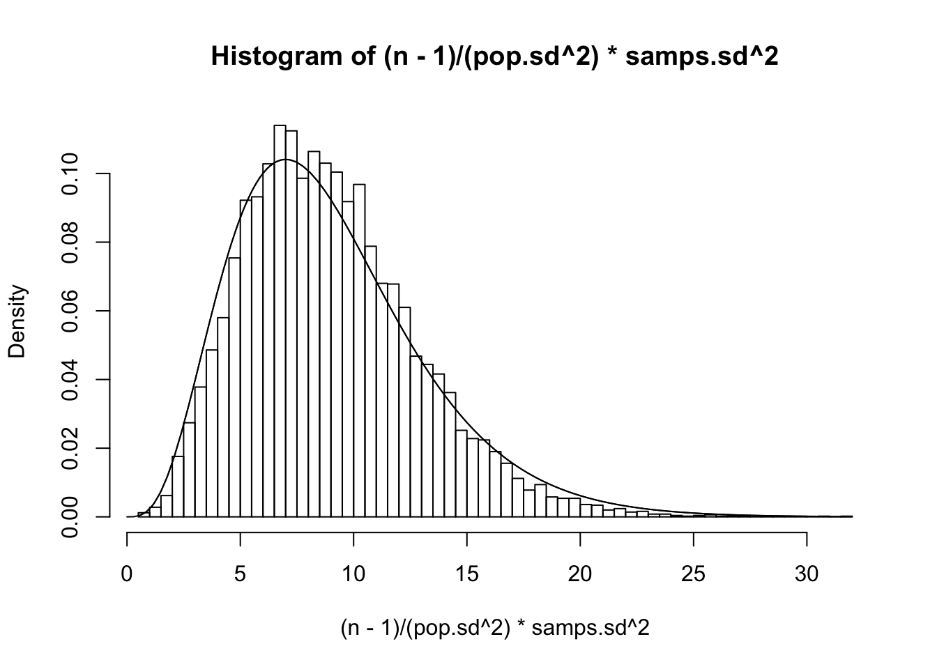

Looks pretty good! Finally, he finds the distribution of the distances of the sample mean to the true mean \(\bar{X_n}-\mu\), divided by the standard deviation of the sample mean \(s/\sqrt{n}\) (instead of dividing by \(\sigma/\sqrt{n}\); see previous post).

\[ t=\frac{\bar{X}-\mu}{s/\sqrt{n}}, \text{ which has the density}\\ p(t|n)=\frac{\Gamma(\frac{n}{2})}{\Gamma(\frac{n-1}{2})} \frac{1}{\sqrt{(n-1)\pi}}\left(1+\frac{t^2}{n-1}\right)^{-n/2} \]

Replacing \(\sigma\) with \(s\) in our Z-score formula gives a statistic that follows …you guessed it, the t distribution! The function itself looks way different that the normal density function \(p(x|\mu,\sigma)=\frac{1}{\sqrt{2 \pi}\sigma}e^{-\frac{(x-\mu)^2}{2\sigma^2}}\). First of all, notice that it doesn’t depend on \(\mu\) or \(\sigma\) at all; let’s see how it actually looks compared to a normal distirbution

t.pdf<-function(x,n){gamma(n/2)/(sqrt((n-1)*pi)*gamma((n-1)/2))*(1+x^2/(n-1))^(-n/2)}
{curve(t.pdf(x,3),xlim=c(-4,4),ylim=c(0,.4),col="red")
  curve(t.pdf(x,4),xlim=c(-4,4),ylim=c(0,.4),col="red",add=T,lty=2)
  curve(t.pdf(x,6),xlim=c(-4,4),ylim=c(0,.4),col="red",add=T,lty=3)
  curve(t.pdf(x,11),xlim=c(-4,4),ylim=c(0,.4),col="red",add=T,lty=4)
  curve(t.pdf(x,26),xlim=c(-4,4),ylim=c(0,.4),col="red",add=T,lty=5)
curve(dnorm(x,0,1),add=T,col="blue")}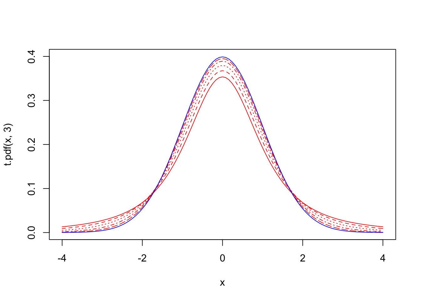

Above, we have plotted five t distributions (red) with 2, 3, 5, 10, and 25 degrees of freedom. Notice that the distribution with df=25 is almost indistinguishable from the normal distribution (blue). In fact, though it wasn’t proven until much later, \(t_n \rightarrow N(0,1)\ as \ n \rightarrow \infty\)

Does this jibe with our observed data better than the normal? Let’s look at our samples of size 3 again and plot their respective t-statistics:

n=3
ts=(samps3.mean-pop.mean)/(samps3.sd/sqrt(n))
{hist(ts,prob=T,breaks=500,xlim=c(-10,10))
curve(dt(x,df=2),add=T,col="red")
curve(dnorm(x,0,samps3.sd[1]/sqrt(n)),add=T,col="blue")}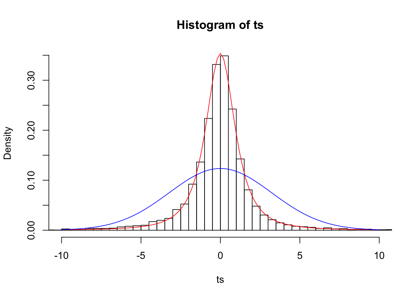

n=10
ts=(samps.mean-pop.mean)/(samps.sd/sqrt(n))
{hist(ts,prob=T,breaks=50,xlim=c(-5,5))
curve(dt(x,df=9),add=T,col="red")
curve(dnorm(x,0,samps.sd[1]/sqrt(n)),add=T,col="blue")}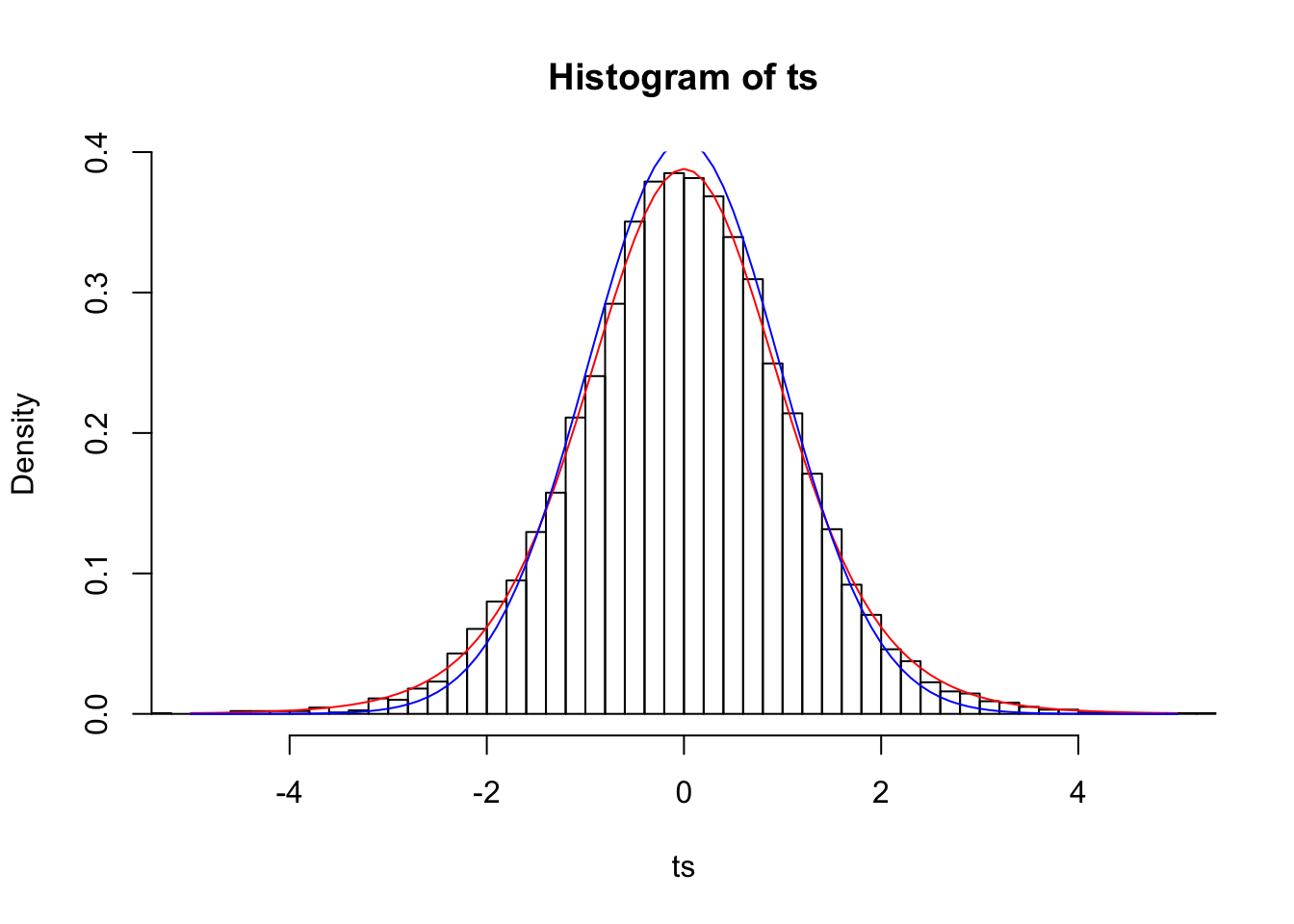

Looks much better! Remember how when we assumed that the means of samples of size 3 were normally distributed, our 95% confidence interval (the interval from Z=-1.96 to Z=1.96) only included the mean 79.41% of the time? In a \(t\) distribution with n-1 degrees of freedom, 95% of the distribution lies within 4.3 sample standard deviations of the population mean.

qt(c(.025,.975),2)

## [1] -4.302653  4.302653

x1<-seq(-6,-4.3,len=100)
x2<-seq(4.3,6,len=100)
y1<-dt(x1,2)
y2<-dt(x2,2)
x3<-seq(-6,-1.96,len=100)
x4<-seq(1.96,6,len=100)
y3<-dnorm(x3)
y4<-dnorm(x4)
{curve(dt(x,2), from=-6, to=6,ylim=c(0,.4),col="red")
curve(dnorm(x),from=-6, to=6,add=T,col="blue")
polygon(c(x1[1],x1,x1[100]),c(0,y1,0),col="red",border=NA)
polygon(c(x2[1],x2,x2[100]),c(0,y2,0),col="red",border=NA)
polygon(c(x3[1],x3,x3[100]),c(0,y3,0),col="blue",border=NA)
polygon(c(x4[1],x4,x4[100]),c(0,y4,0),col="blue",border=NA)}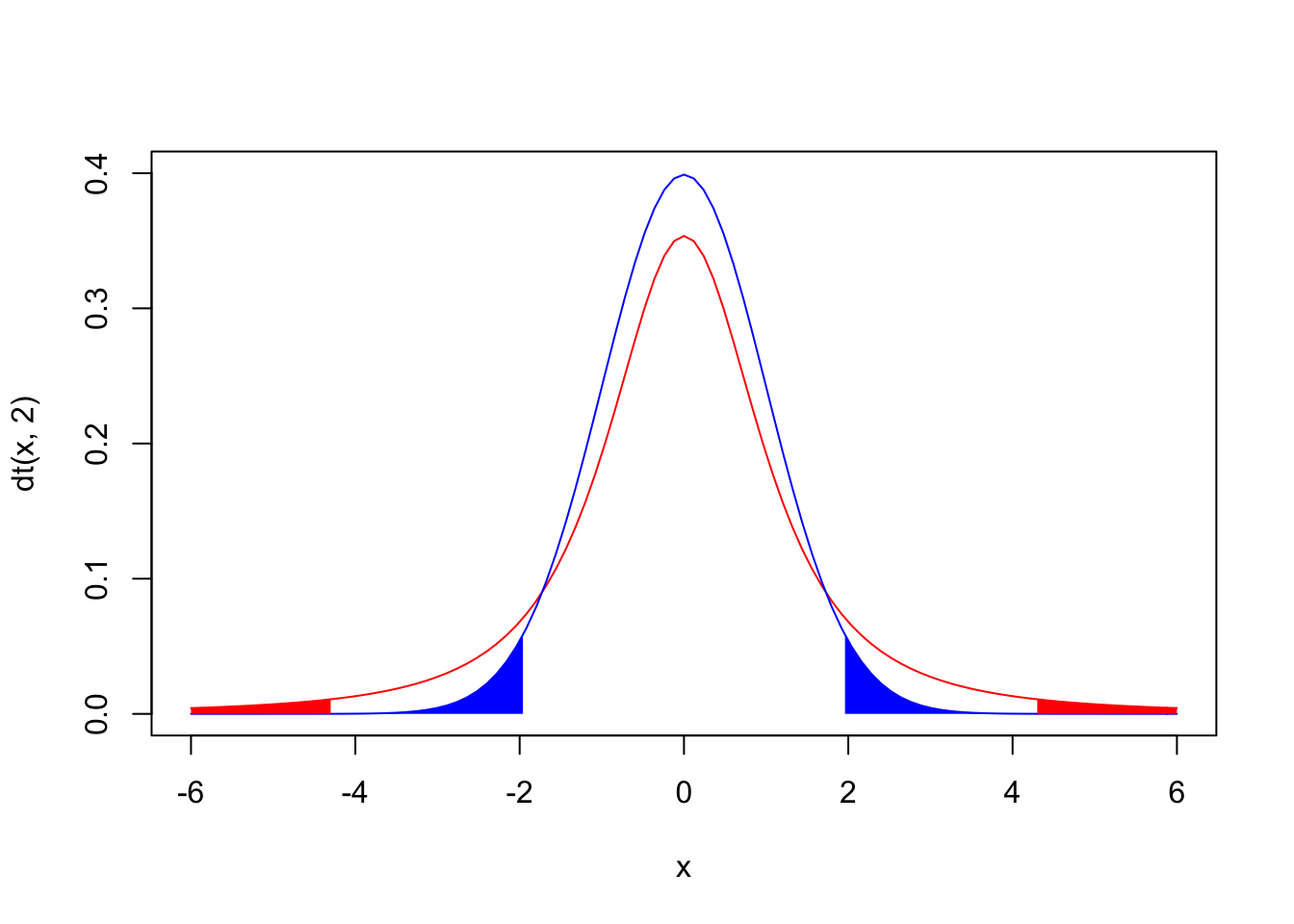

The plot above shows a normal \(N(0,1)\) distribution in blue and a \(t\) distribution with 2 degrees of freedom in red; note that the red areas under the \(t\) add up to 5% and the blue areas under the \(N(0,1)\) add up to 5%.

Since the \(t\)-statistic \(t=\frac{\bar{X}-\mu}{s/\sqrt{n}}\) follows this distribution, we can rearrange it to find the confidence interval around the population mean.

\[ -t \le \frac{\bar{X}-\mu}{s/\sqrt{n}} \le t \\ \frac{-ts}{\sqrt{n}} \le \bar{X}-\mu \le \frac{ts}{\sqrt{n}} \\ \frac{-ts}{\sqrt{n}}-\bar{X} \le -\mu \le \frac{ts}{\sqrt{n}}-\bar{X} \\ \frac{ts}{\sqrt{n}}+\bar{X} \ge \mu \ge \frac{-ts}{\sqrt{n}}+\bar{X} \\ \bar{X}-\frac{ts}{\sqrt{n}} \le \mu \le \bar{X}+\frac{ts}{\sqrt{n}} \]

Lets create 10,000 intervals just like the one above using random draws from our population of heights to find our \(\bar{X}\) and s to see how many times they don’t actually contain the true mean \(\mu\). We will use \(t=4.3\) because we saw that if the sample means follow a t-distribution, the 95% of the density should be within \(\bar{X}\pm 4.3\) sample standard deviations (\(s/\sqrt{n}\)) away.

samps3t<-matrix(nrow=3,ncol=10000)
samps3t<-replicate(10000,sample(pop.height,3,replace=T))
samps3t.mean<-apply(samps3t,2,mean)
samps3t.sd<-apply(samps3t,2,sd)
s3t.s<-mean(samps3t.mean-4.303*samps3t.sd/sqrt(3)> pop.mean | pop.mean>samps3t.mean+4.303*samps3t.sd/sqrt(3))
s3t.s

## [1] 0.056

Yay! Assuming a t-distribution, the population mean falls outside our 95% confidence interval 5.6% of the time; clearly this distribution is a much better fit for a sampling distribution when samples are small and we are using \(s\) instead of \(\sigma\).

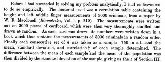
#Student’s “Simulations”

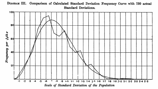
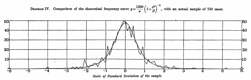
Thanks to computers, we can easily check the results of our derivations by using monte carlo sampling techniques. Gosset obviously could not do this. Perhaps the most remarkable thing about his paper, however, is that it does contain one of the earliest simulation studies in history. He did this by hand, with “3000 pieces of cardbord, which were very thoroughly shuffled and drawn out at random.”

Below, he plots the observed distribution of the standard deviations of his samples of size \(n=4\) and overlays his curve:

And here below, he plots his observed distribution of \(z=\frac{\bar{X}-\mu}{s/\sqrt{n}}\), where his \(s\) divides by \(n\) instead of \(n-1\),

#Hypothesis Testing with the T-Test

The development of the t distribution was hugely important because it gave the enabled the t-test, commonly used as a location test for the mean. Recall that the t statistic \(t=\frac{\bar{X}-\mu}{\sigma/\sqrt{n}}\) follows a t-distribution (with \(n-1\) degrees of freedom). Now, given that we have some data, the only unknown here is the parameter \(\mu\), the population mean. Let’s generate a null hypothesis: let \(\mu=\mu_0=0\) and \(n=10\); this gives a distribution of the sample mean \(\bar{X}\) for samples of size 10 around a “true” population mean of \(\mu_0=0\), while accounting for uncertainty in the sample variance. Thus, we can ask how likely we are to observe our sample mean \(\bar{X}_{10}\), given that the true population mean is actually 0. Let’s do this; we will take a random sample of size from a normal distribution with a mean of 1 and a standard deviation of 1; we will then calculate the mean and ask how likely this value would be if the true mean was actually equal to 0.

tsamp<-rnorm(10,1,1)
tsamp.mean<-mean(tsamp)
tsamp.sd<-sd(tsamp)
tstat<-(tsamp.mean-0)/(tsamp.sd/sqrt(10))
x1<-seq(-5,-2.26,len=100)
x2<-seq(2.26,5,len=100)
x3<-seq(tstat,5,len=100)
x4<-seq(-5,-1*tstat,len=100)
y1<-dt(x1,9); y2<-dt(x2,9); y3<-dt(x3,9);y4<-dt(x4,9)
{curve(dt(x,9),main="",xlim=c(-4,4))
polygon(c(x1[1],x1,x1[100]),c(0,y1,0),col="grey",border=NA)
polygon(c(x2[1],x2,x2[100]),c(0,y2,0),col="grey",border=NA)
polygon(c(x3[1],x3,x3[100]),c(0,y3,0),col="black",border=NA)
polygon(c(x4[1],x4,x4[100]),c(0,y4,0),col="black",border=NA)
abline(v=tstat,lty=2)}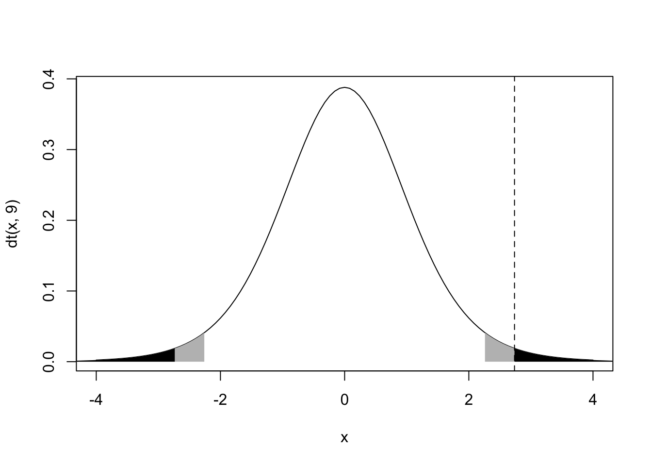

2*(1-pt(tstat,df=9))

## [1] 0.02300813

The probability of observing a sample mean (i.e., a t statistic) at least this extreme (in either direction!) is .016 (this is the sum of the black areas under the t curve). The area under the curve to the right of our observed statistic is only round(1-pt(tstat,df=9),3), but we have to double it to account for a just as extreme or more extreme observation happening in the other direction. We do this because we didn’t have any a priori hypothesis about the direction of the effect: our default alternative hypothesis was that \(\mu \ne 0\), or \(prob \gt |t|=p \lt -t + p > t\) where t is our observerd t-statistic tstat. The area shown in gray plus the area in black is equal to 5% of the distribution, 2.5% on each side. This represents the standard “rejection region” with a significance level of 0.05; thus, even if the null hypothesis is true and there is no effect (i.e., \(\mu =0\)), 5% of the time we would still observe sample means that are at least this extreme: namely, more than \(t^*_{(1-\frac{\alpha}{2}=.975,n-1=9)}=2.262\) sample standard deviation away from the true mean.

Assumptions: Independence, Normality, and Equality of Variances

When the t-test is used to compare samples from two populations, the main assumptions that need to be met for this purpose are that the populations are (1) independent of one another, are (2) both normally distributed, and (3) both have the same variance. The first of these can often be fixed using a paired t-test (see below). The second–normality–is usually met in practice thanks to the central limit theorem, but if non-normality is a problem then non-parametric tests such as the Mann-Whitney U test can be used instead. The third–unequal variances–can be tricky, but there are fixes here as well (see Welch’s t-test below).

In order to test for differences between two sample means, we need to find the distribution of \(\bar{X}_1 - \bar{X}_2\). For large samples (or when we know the populations are normal), we find that \(\bar{X}_1 - \bar{X}_2\) is normally distributed, with a mean of \(\mu_1-\mu_2\) and a pooled variance equal to \(\sqrt{\frac{\sigma_1^2}{n_1}+\frac{\sigma_2^2}{n_2}}\). But when we don’t know \(\sigma\) (which is like, always) and when samples are small (< 30 or so, which is common), this becomes a t-test. Assuming the independence, normality, and equal variance (a.k.a. homoscedasticity) assumptions are met, you would compare two groups with sample means \(\bar{X}_1, \bar{X}_2\), sample standard deviations \(s_1, s_2\), and sample sizes \(n_1, n_2\) using the statistic \(t=\frac{\bar{X}_1-\bar{X}_2}{s_p \sqrt{\frac{1}{n_1}+\frac{1}{n_2}}}\), where \(s_p\) equals \[ s_p=\sqrt{\frac{(n_1-1)s_1^2 + (n_2-1)s_2^2}{n_1+n_2-2}} \]

Derivation

He begins by deriving the distribution of the sample standard deviation s for samples of a given size n drawn from a standard normal distribution. If \(x_1, x_2, ...,x_n\) is one of these samples then, using a property we derived in the previous post, for one sample we have

\[ \begin{align} s^2&=\frac{\sum(x_i^2)}{n}-\left(\frac{\sum(x_i)}{n}\right)^2\\ &= \frac{\sum(x_i^2)}{n} - \frac{\sum(x_i^2)}{n^2} - \frac{2\sum_{i<j}(x_ix_j)}{n^2}\\ \end{align} \] So the expected value of the standard deviation across all such samples is \[ \begin{align} E\left[s^2\right]&=E\left[\frac{\sum(x_i^2)}{n} - \frac{\sum(x_i^2)}{n^2} - \frac{2\sum_{i<j}(x_ix_j)}{n^2}\right]\\ &=\frac{\sum E[x_i^2]}{n}-\frac{\sum E[x_i^2]}{n^2}-\frac{2\sum_{i<j}E[x_ix_j]}{n^2} \\ &= \frac{n\mu'_2}{n}- \frac{n\mu'_2}{n^2}-0 \text{ , (since independent, }E[x_ix_j]=E[x_i]E[x_j]=0\times 0\text{)}\\ &=\frac{\mu'_2(n-1)}{n} ,\text{ where }\mu'_2 =E[x_i^2], \text{the second moment.} \end{align} \] The he says OK, so we’ve got the expected value, or the mean, of \(s^2\). He goes on to find, “in the same tedious way,” that the means of \(s^4, s^6, s^8\) are \[ \begin{align} E[s^4] &= (\mu'_2)^2 \frac{(n-1)(n+1)}{n^2}, \\ E[s^6] &= (\mu'_2)^3 \frac{(n-1)(n+1)(n+3)}{n^3}, \\ E[s^8] &= (\mu'_2)^4 \frac{(n-1)(n+1)(n+3)(n+5)}{n^4},\\ ... \end{align} \] These are raw moments. To find the central moments of s^2 about its mean (that is, to find the variances), we do so in this way \[ \begin{align} M_2 &=E\left[(s^2-E[s^2])^2\right]=V[s^2]=E[(s^2)^2]-\left(E[s^2]\right)^2= \\ &= E[(s^4)]-\left(E[s^2]\right)^2 \\ &= (\mu'_2)^2 \frac{(n-1)(n+1)}{n^2} - \left(\frac{\mu'_2(n-1)}{n} \right)^2 \\ &= (\mu'_2)^2 \frac{(n-1)(n+1)}{n^2} - \frac{(\mu'_2)^2(n-1)^2}{n^2} \\ &= (\mu'_2)^2\frac{(n-1)}{n^2}\left[(n+1)-(n-1) \right] \\ &= 2 (\mu'_2)^2\frac{(n-1)}{n^2}, \text{ remembering that }\mu'_2=E[x_i^2]. \end{align} \] When you find the other moments \(M_3=V[s^4]\) and \(M_4=V[s^6]\), you get \[ \begin{align} M_3&=V[s^4]=8(\mu'_2)^3\frac{(n-1)}{n^3},\\ M_4&=V[s^6]=12(\mu'_2)^4\frac{(n-1)(n+3)}{n^4} \end{align} \] Now it’s time to pause for a second. It turns out that Karl Pearson, STUDENT’s mentor, had already discovered the t-distribution in 1895/1901 (along with the gamma distribution and several others). Pearson parameterized his distributions using two quantites: \(\beta_1 = \gamma_1^2\) (where \(\gamma_1\) is the skewness, or third standardized moment) and \(\beta_2=\gamma_2+3\), where \(\gamma_2\) is traditional kurtosis. Here, \[ \gamma_1=E\left[\left(\frac{s^2-E(s^2)}{\sqrt{Var[s^2]}}\right)^3\right]=\frac{M_3}{\sqrt{M_2^3}} \] So \[ \beta_1=\gamma_1^2=\frac{M_3^2}{M_2^3}=\frac{8^2(\mu'_2)^6\frac{(n-1)^2}{n^6}}{2^3 (\mu'_2)^6\frac{(n-1)^3}{n^6}}=\frac{8}{n-1} \] And \[ \beta_2=\gamma_2=E\left[\left(\frac{s^2-E(s^2)}{\sqrt{Var[s^2]}}\right)^4\right]=\frac{M_4}{M_2^2}=\frac{12(\mu'_2)^4\frac{(n-1)(n+3)}{n^4}}{2^2 (\mu'_2)^4\frac{(n-1)^2}{n^4}}=\frac{3(n+3)}{n-1} \]

To make a long story short, he realized that the four moments he computed, scaled in this way, corresponded to one of Pearsons equations (which were parametrized withvalues of \(\beta_1\) and \(\beta_2)\). Can you find which one? For instance, when \(n=2\), \(\beta_1=8\) and \(\beta_2=15\)

STUDENT: “Consequently, a curve of Professor Pearson’s type III maybe expected to fit the distribution of s^2.” The curve in questions is \(y=Cx^pe^{-\gamma x}\), where \(\gamma=2\frac{M_2}{M_3}=\frac{n}{2\mu'_2}\) and \(p=\frac{4}{\beta_1}-1=\frac{n-3}{2}\), thus yielding \[ y=Cx^{\frac{n-3}{2}}e^{\frac{nx}{2\mu'_2}} \] “Which will give the distribution of \(s^2\)” (i.e., \(x=s^2\))

Great, so now we’ve got our sampling distribution for the standard deviation! Recalling that the sampling distribution for the sample mean is just normal—\(N(\mu,\frac{\sigma}{\sqrt{n}})\), \[ y=\frac{1}{\sqrt{2\pi}(\sigma/\sqrt{n})}e^{-\frac{x^2}{2(\sigma/\sqrt{n})^2}} \]

He says, “now let us suppose \(x\) [which, recall, are observations measured as distances from the population mean] is measured in terms of \(s\), i.e. let us find the distribution of \(z=\frac{x}{s}\)” which gives,

\[ y=\frac{s}{\sqrt{2\pi}(\sigma/\sqrt{n})}e^{-\frac{s^2z^2}{2(\sigma/\sqrt{n})^2}} \]

To be continued (sorry y’all, this is taking me forever)… at this point I want to just do a change of variable and integrate but that’s not how he does it (at least… I don’t think so?)