
Hello! This is the first in a series of posts that cover topics typically encountered on any Introduction to Statistics course syllabus (yes, that is to say frequentist). The idea was born out of a desire to blog about the Analysis of Variance and its many forms, but I soon found myself addressing pre-requisites, which led to tangents and lemmas that took on lives of (and ballooned into posts of) their own. So here were are, getting our feet wet with sampling distributions (in which the Law of Large Numbers (LLN) and the Central Limit Theorem (CLT) play leading roles). These two grand-sounding acronyms are just as grand as they sound, so hold on to your ass! If you have already been initiated into the mysteries of LLN/CLT, you are heartily encouraged to skip ahead.
Introduction: Concrete Example
Alright then, let’s say you want to know the average height of all undergraduate students at the University of Texas at Austin. However, we don’t want to measure all ~40,000 students, so we take a sample, take the average height, and hope that it is close to the average height of all students. But how close is it?
Let’s pretend this is our population. Because male and female heights follow different normal distributions, we will approximate a population like this (I pulled these params from wolfram alpha).
set.seed(9999)
pw<-.515
women.height<-rnorm(pw*40000,63.8,2.7)
men.height<-rnorm((1-pw)*40000,69.3,3.0)
pop.height<-c(women.height,men.height)
pop.mean<-mean(pop.height)
pop.sd<-sd(pop.height)
hist(pop.height,prob=T,breaks=100,main = "")
curve(dnorm(x,pop.mean,pop.sd), add=TRUE)
curve(dnorm(x,63.8,2.7)/(1/pw),add=T,col="red")
curve(dnorm(x,69.3,3.0)/(1/(1-pw)),add=T,col="blue")
curve(dnorm(x,63.8,2.7)/(1/pw)+dnorm(x,69.3,3.0)/(1/(1-pw)),add=T,col="green")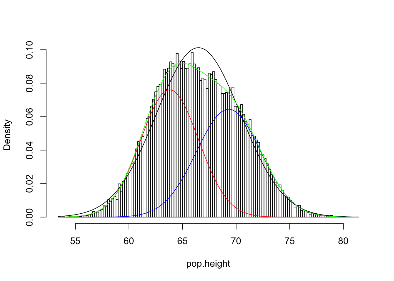
The population (green) is not quite normal; rather, it’s a mix of two normal distributions: see red and blue normals. Add them together, and you get the green one. The mean and standard deviation of our population are 66.49 and 3.94, and a normal distribution with those parameters is shown in black. But lets forge ahead and see what happens; we grab the first student who passes by and we measure them. Remember, we are interested in the average height of all students!
s1<-sample(pop.height,1,replace=T)
s1
## [1] 66.25691Since all we have is this one student’s height, this is our best estimate of the population mean. But how sure are we? Is this a good estimate? Remember (wink-wink), we don’t actually know the mean or standard deviation of our population. As it stands, we have no way of quantifying our uncertainty. What can we say about the population mean with a sample size of 1? (Answer: not much?!)
Bumping into the Law of Large Numbers
We would like to have a better estimate of the mean, and we need some way of quantifying our uncertainty, so lets collect more data. We measure 10 people this time, and take the mean and standard deviation.
s10<-sample(pop.height,10,replace=T)
mean(s10);sd(s10)
## [1] 68.7775## [1] 3.660682Well—becoming omnicient for a moment—we can see that this mean is quite a bit closer to the population mean:\(\mid \bar{X}_{10}-\mu\mid=\) 2.292 versus \(\mid \bar{X}_1-\mu\mid=\) 0.228. Are we guaranteed to get closer and closer to the population mean as we measure more and more people?
ss<-vector()
ss[1]<-s1
for(i in 2:1000){
  ss[i]=mean(sample(pop.height,i,replace=T))
}
plot(ss,type='l',ylab="mean of sample", xlab="sample size")
abline(pop.mean,0,col="green")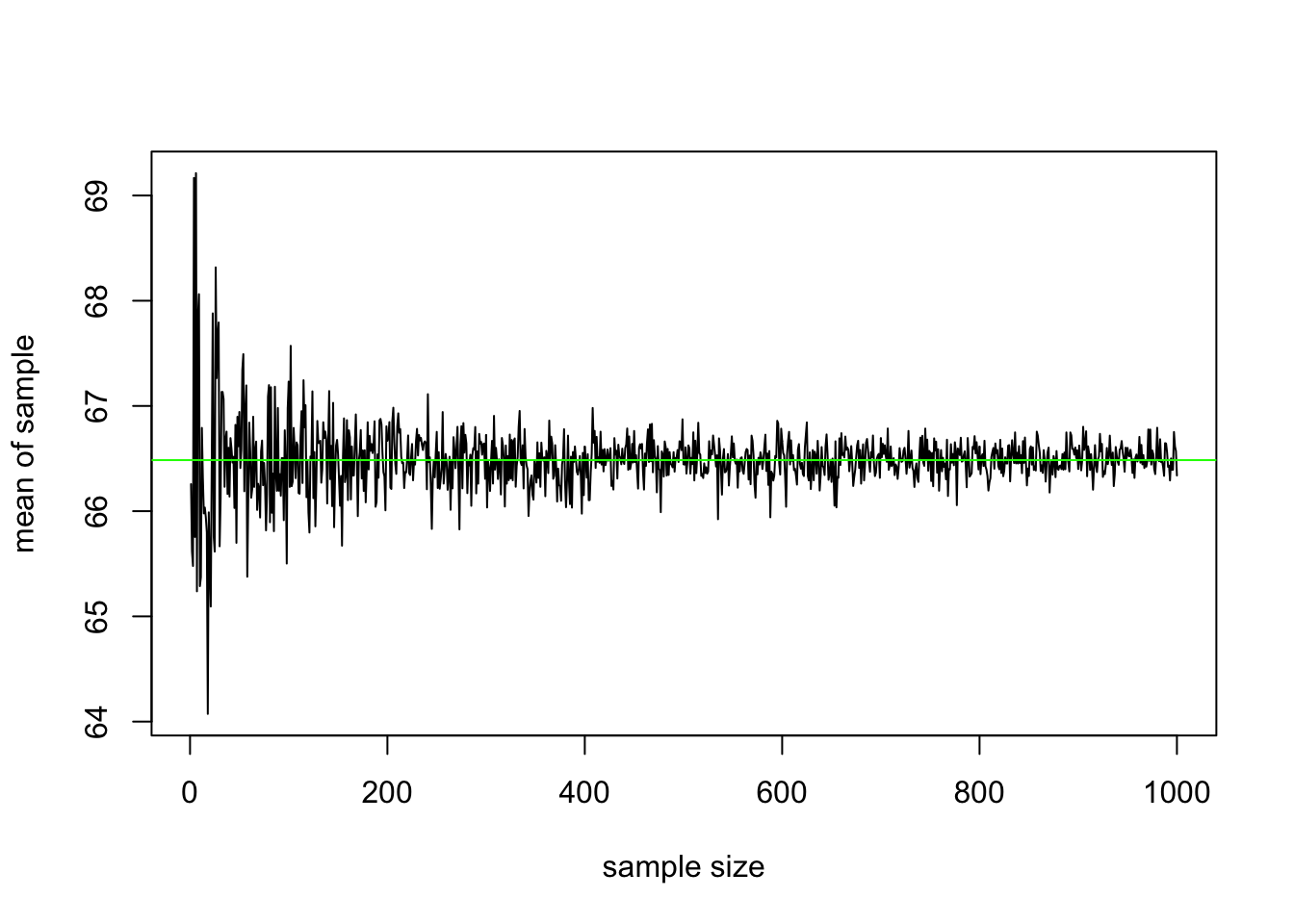
It appears so! Namely, we claim that the sample average \(\bar{X}_n = \frac{1}{n}(X_1+...+X_n)\) of independent observations from the same distribution converges to the mean of the distribution \(\mu\). That is, as \(n \rightarrow \infty\), \(\bar{X}_n \rightarrow \mu\). This is a form of the Law of Large Numbers: essentially, the average of more and more (i.i.d.) variables gets closer and closer to a single number, the expected value (or population mean). We will prove it later, when we have another tool to help us!
Standard Deviation of the Sample Mean (aka “Standard Error”)
OK, so we know that our sample mean is a good estimator of the population mean, especially if we have a large sample, but let’s not be hasty. What does this tell us? Well, the mean of the sample of 10 heights is 68.78 and the standard deviation is 3.66; we know that for a normal distribution, ~95% of the data lies within two-ish (1.96) standard deviations above and below the mean. Does this mean that we are 95% sure that the population mean lies within
c(mean(s10)-1.96*sd(s10), mean(s10)+1.96*sd(s10))## [1] 61.60256 75.95244Unfortunately, no. This is the sample standard deviation of heights: how far our 10 heights are away from their own mean on average. But the individual heights don’t concern us: we are interested in the mean! How close is our mean to the population mean? To get at this, we need to know how the sample mean itself is distributed instead of the individual observations. We can’t expect the mean to have the same distribution as the original distribution! That is, if we took tons of random samples of 10 people and took the average height for each sample, what sort of a distribution would these means follow? Would it be normal? Would it be more or less spread out than the original distribution? Let’s have a look
samps10<-replicate(10000,sample(pop.height,10,replace=T))
s10.means<-apply(samps10,2,mean)
hist(s10.means,breaks=20,prob=T,main="",xlim=c(60,73))
curve(dnorm(x,mean(s10.means),sd(s10.means)),add=T)
curve(dnorm(x,63.8,2.7)/(1/pw)+dnorm(x,69.3,3.0)/(1/(1-pw)),add=T,col="green")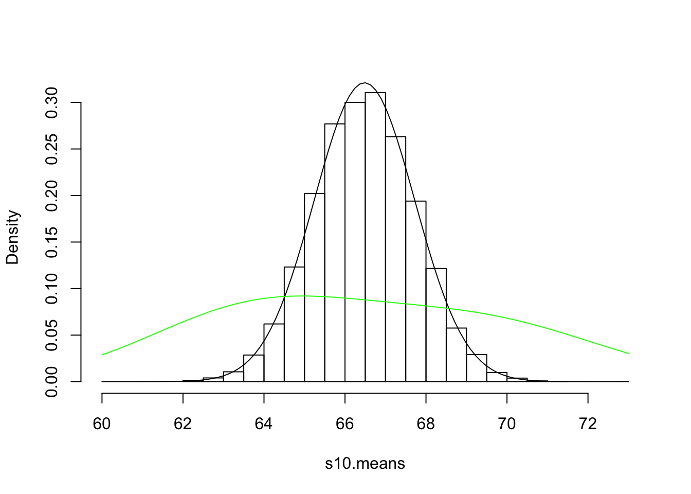
Now, I ask you: what is the standard deviation of these 10-observation means?
sd(s10.means)## [1] 1.242055Quite small! Quite a bit smaller than our original sample standard devation 3.66 (and—omnisciently again—quite a bit smaller than our population sd of 3.94). Just look at the overlayed population distribution (green), or compare range of the distribution of the sample means (62.02, 71.03) to the range of the population (53.42, 81.28)! How about the mean?
mean(s10.means)## [1] 66.48131Pretty close to the mean of our first sample of 10, 68.78, and right on top of the population mean, 66.49 as expected. So when we take a bunch of samples of a certain size and we take their means, the mean of those means will approach the population mean (LLN), but the standard deviation of those means doesn’t approach the population standard deviation. Why? What does it approach?
Averages are—by definition—right in the middle of a sample, so means are always less extreme than the observations they are based on. This explains why we saw that our distribution of means had a tighter range and sd than the population it is based on. Now, the smaller the sample, the more likely your mean is to be skewed one way or another by the influence of extreme observations you randomly chose. Conversely, when each sample is larger, it is more representative, and thus extreme observations are given less weight each time you take the mean. Recall the mean of our first sample of 10, 68.78. This was 2.292 away from the population mean. But if we took a sample of 100, the mean of this sample should be much closer.
s100<-sample(pop.height,100,replace=T)
abs(mean(s100)-pop.mean)
## [1] 1.236596And it is. If we took a bunch of 100-person samples and took the mean of each one, these means will be much closer together than the means of 10-person samples: that is, their variance (and sd) will be smaller. Here’s proof:
samps100<-replicate(10000,sample(pop.height,100,replace=T))
s100.means<-apply(samps100,2,mean)
hist(s100.means,breaks=20,prob=T,main="",xlim=c(60,73))
curve(dnorm(x,mean(s100.means),sd(s100.means)),add=T)
curve(dnorm(x,63.8,2.7)/(1/pw)+dnorm(x,69.3,3.0)/(1/(1-pw)),add=T,col="green")
curve(dnorm(x,mean(s10.means),sd(s10.means)),add=T)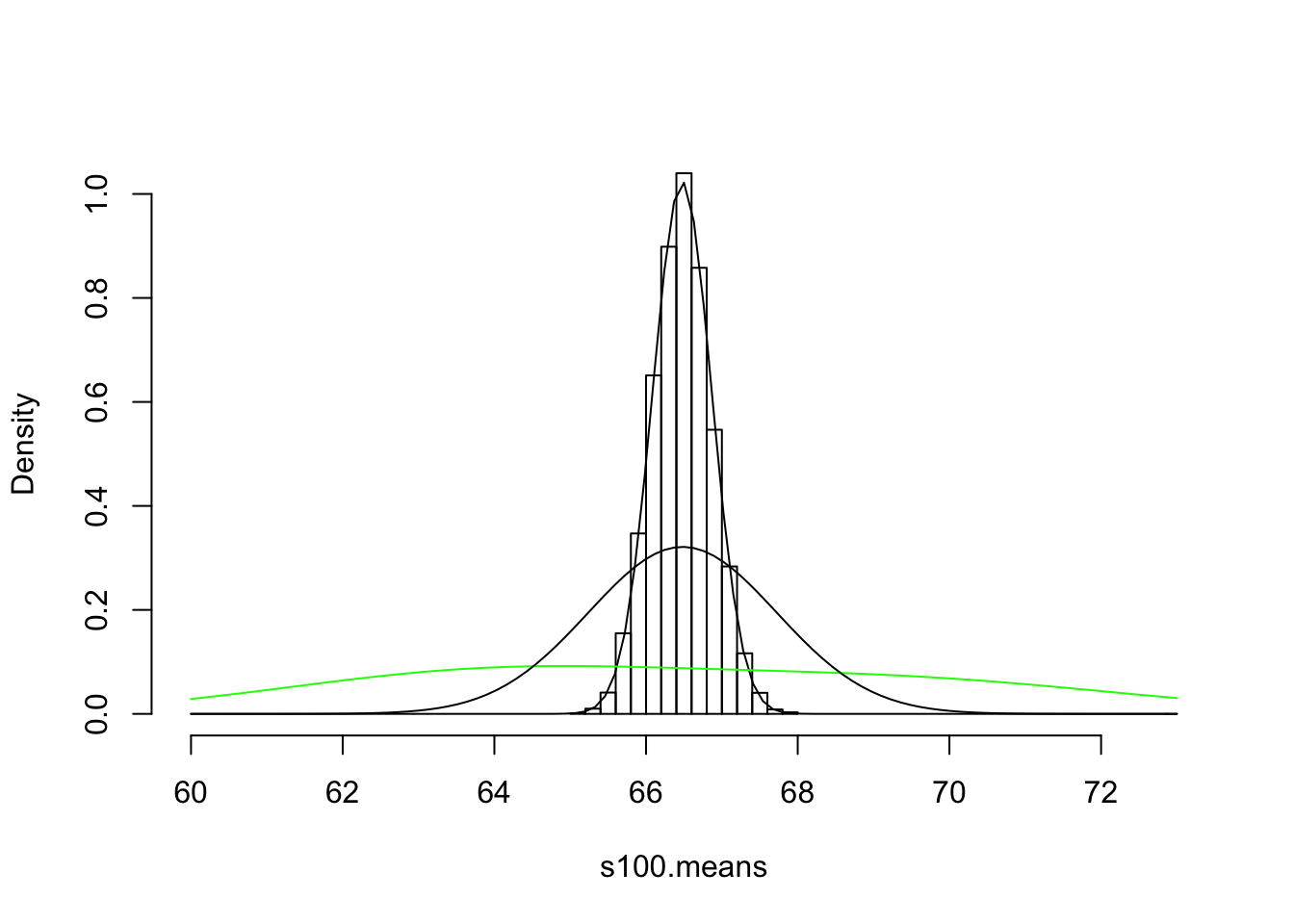
sd(s100.means)## [1] 0.3897787So the variance of the distribution of means \(\bar{X}\) is a function of the size of the sample each mean is based on. That’s reasonable: taking it to it’s logical conclusion, if you were to take a bunch of samples of 40,000 people from our population of 40,000 then the mean of each sample will always equal the population mean, and thus the variance of all of these means will be zero.
What exactly is the relationship between sample size and the standard deviation of the sample mean? We will prove this mathematically below, but for let’s just brute force it: we will take 1000 samples of size 2 and take the average of each, 1000 samples of size 3 and take the average of each, all the way up to sample of size 500. Then, we will plot the standard deviation of the 1000 sample means for each sample size.
samps.big<-matrix(nrow=500,ncol=1000)
for(n in 1:500){
  samps.big[n,]<-replicate(1000,mean(sample(pop.height,n,replace=T)))
}
samp.sds<-apply(samps.big,1,sd)
plot(samp.sds,type='l',ylab="SD of sample mean", xlab="sample size",ylim=c(0,4))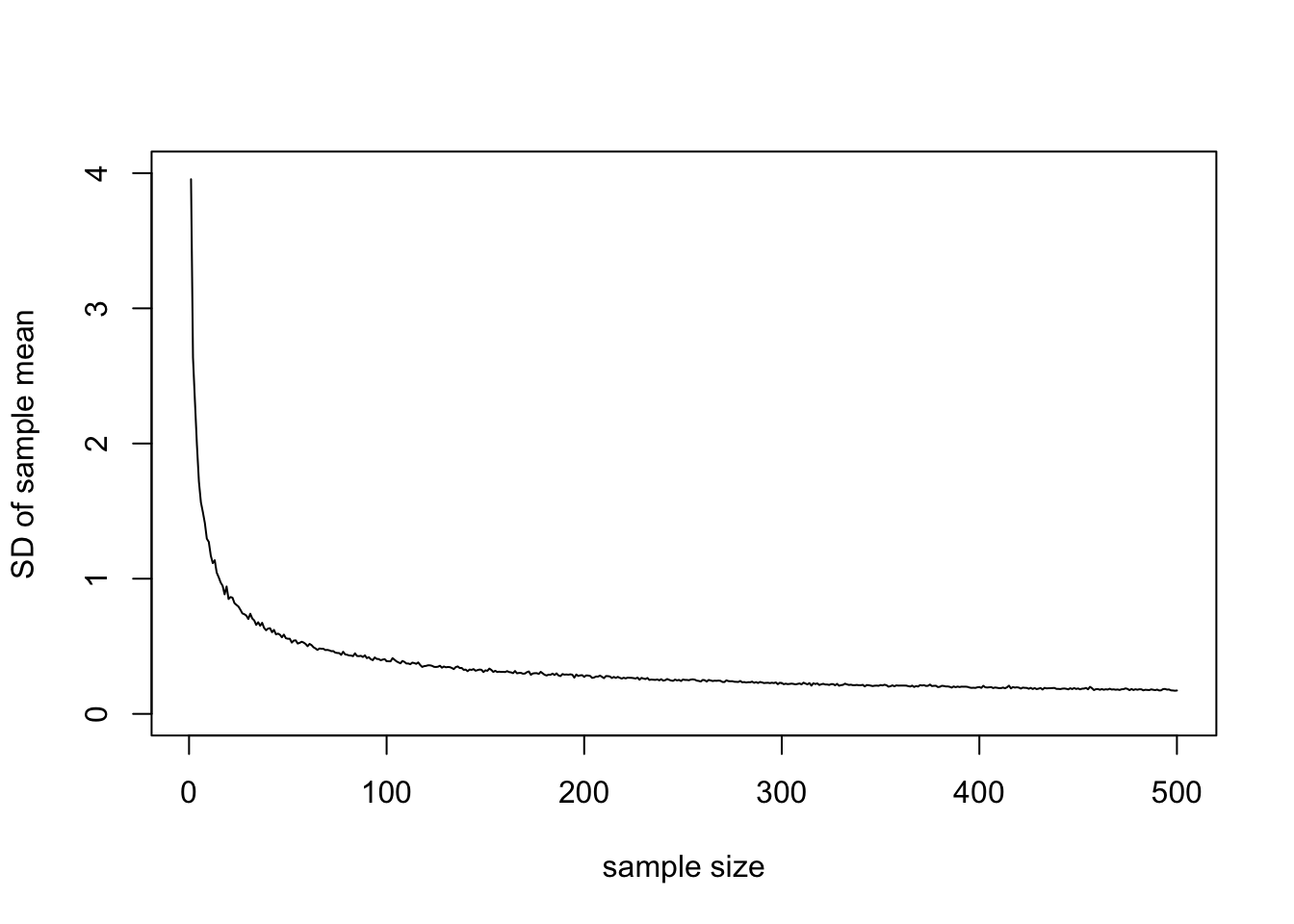
As we suspected, the standard deviation of the sample mean approaches 0 as the sample size increases. Let’s look at these sampling distributions of the mean using the new package ggjoy:
## Loading required package: ggridges##
## Attaching package: 'ggridges'## The following object is masked from 'package:ggplot2':
##
## scale_discrete_manual## The ggjoy package has been deprecated. Please switch over to the
## ggridges package, which provides the same functionality. Porting
## guidelines can be found here:
## https://github.com/clauswilke/ggjoy/blob/master/README.mdsamps.big<-as.data.frame(cbind(seq(1,1000,1),t(samps.big)))
names(samps.big)<-c("V1",seq(1,500,1))
samps.thin<-samps.big[,c(1,2,3,6,11,51,101,251,501)]
samps.thin<-melt(samps.thin,id="V1")
names(samps.thin)<-c("id","n","Means")
ggplot(samps.thin, aes(x =Means, y=n,height=..density..))+geom_joy(scale=3)## Picking joint bandwidth of 0.309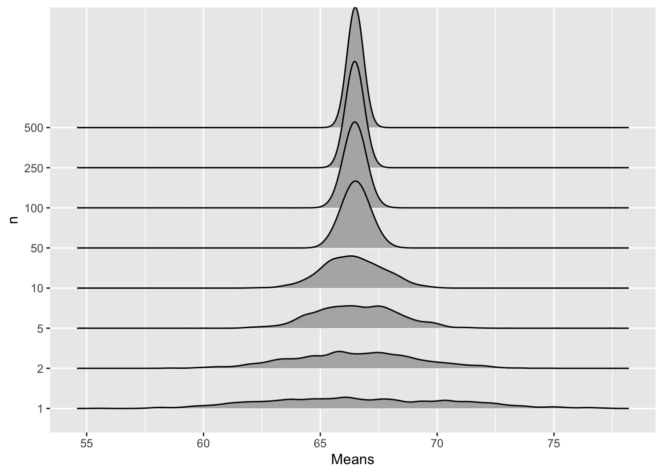
OK fine, so we see its going to zero, but at what rate? Well, we know it’s a function of the population standard deviation, but how exactly are they related? As sample gets bigger, sd gets smaller, so perhaps they are just inversely related (red)? Nope, inverse drops too quickly, but that’s the right idea. We need to make the denominator smaller so it doesn’t drop so much. We can make it smaller by taking the log (blue), or taking the sqare root (green)
plot(samp.sds,type='l',ylab="SD of sample mean", xlab="sample size")
curve(pop.sd/x,add=T,col="red")
curve(pop.sd/log(x),add=T, col="blue")
curve(pop.sd/sqrt(x),add=T,col="green")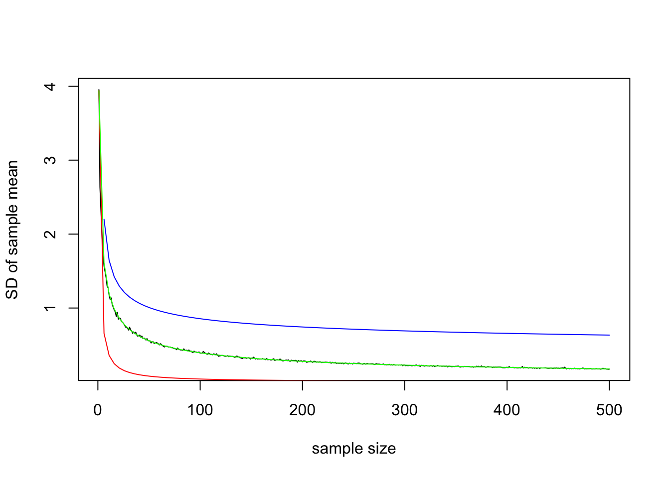
Bingo. The standard deviation of the sample mean appears to be the population standard deviation divided by the square root of the sample size: \(SD(\bar{X})=\frac{\sigma}{\sqrt{n}}\) and thus \(Var(\bar{X})=\frac{\sigma^2}{n}\) as shown below. Note that in both cases, as \(n \rightarrow \infty\), \(Var(\bar{X}) \rightarrow 0\)
plot(samp.sds^2,type='l',ylab="Variance of sample mean", xlab="sample size")
curve(var(pop.height)/x,add=T,col="green")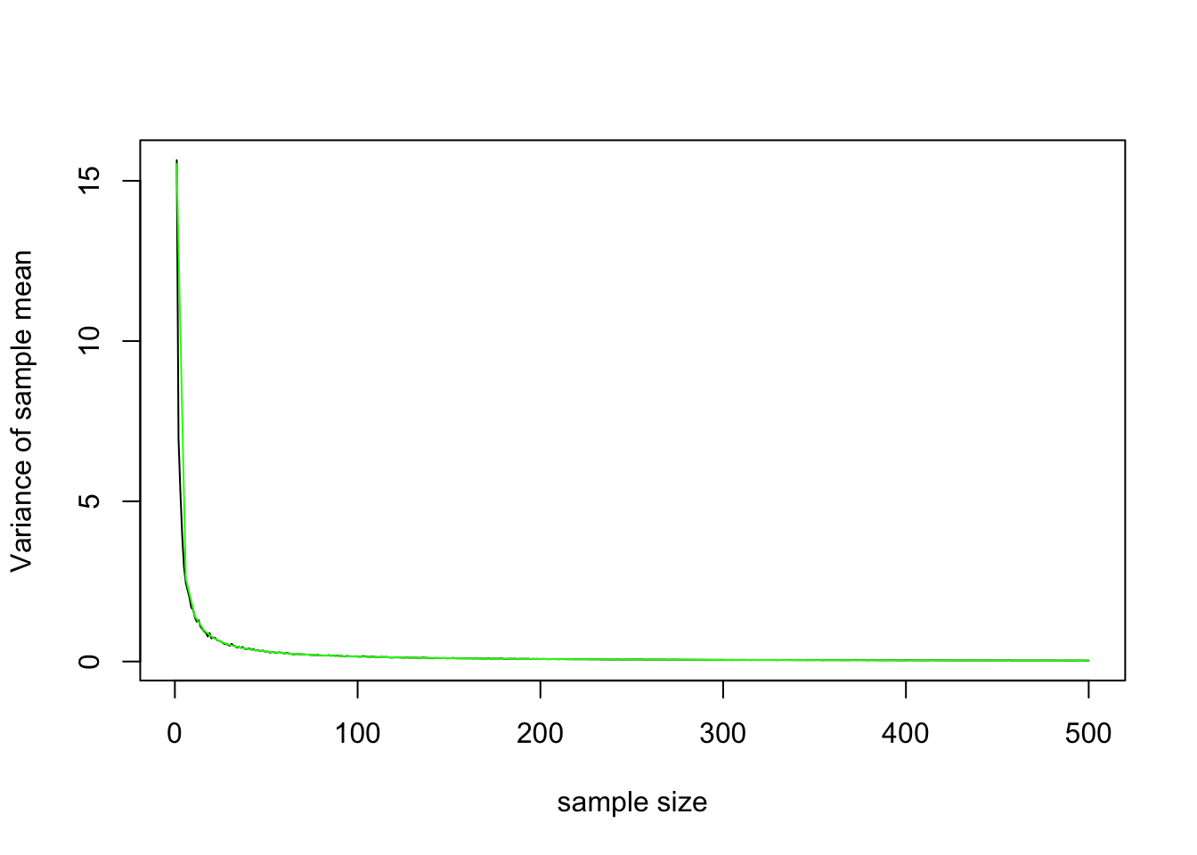
Let’s quickly prove this. We need only invoke two other results: pulling constants out of a \(Var[...]\) squares them, and \(X_is\) from the same distribution have the same \(Var[X_i]=\sigma^2\).
\[ \begin{aligned} Var[\bar{X}] &= Var\left[\frac{X_1+X_2+...+X_n}{n}\right] \\ &= Var\left[\frac{1}{n}X_1+\frac{1}{n}X_2+...+\frac{1}{n}X_n\right] \\ &=\frac{1}{n^2}Var[X_1]+\frac{1}{n^2}Var[X_2]+...+\frac{1}{n^2}Var[X_n] \\ &=\frac{1}{n^2}(\sigma^2+\sigma^2+...+\sigma^2) \\ &=\frac{1}{n^2}(n\sigma^2)\\ &=\frac{\sigma^2}{n} \\ \end{aligned} \]
So now we know that, for samples of a given size \(n\), the means of the samples are normally distributed around the population mean, with a standard deviation of \(\sigma/\sqrt{n}\).
The Central Limit Theorem, Briefly
Perhaps the most amazing part of all this is that the original distribution of the data doesn’t need to be normal for the sampling distribution of the mean to be normal: indeed, it will work with any distribution you want (provided it has finite variance).
For instance, even though in our heights example above the original data wasn’t quite normal (actually coming from mixture of two normals), the mean of samples drawn from this distribution was clearly normal. Here’s a quick, more extreme demonstration for the skeptics among you.
Imagine we have a discrete probability distribution, where are random variable \(X\) can take on three values \(X \in \{-1,0,1\}\) with equal probability:
tab=cbind(X=c(-1,0,1),Prob=c(1/3,1/3,1/3))
tab
## X Prob
## [1,] -1 0.3333333
## [2,] 0 0.3333333
## [3,] 1 0.3333333plot(tab,pch=19,cex=2)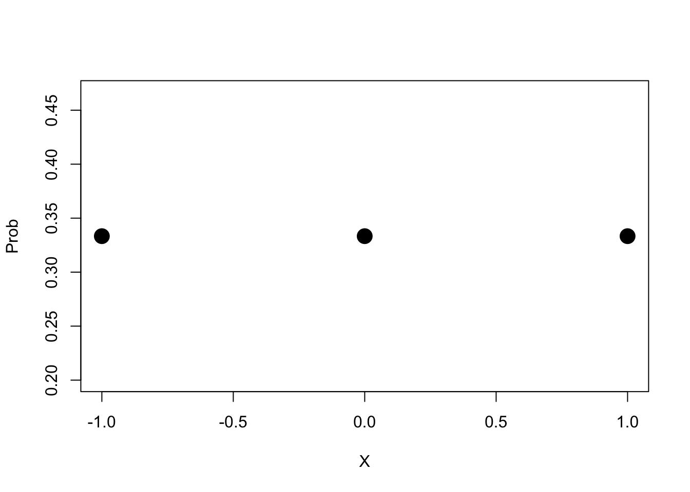
What is the average, or expected value, of \(X\)? \(E[X]=\frac{1}{3}(-1)+\frac{1}{3}(0)+\frac{1}{3}(1)=0\). What is the variance? This is good trick to know so I will write it out in full, but dont worry if you don’t follow it \[ \begin{aligned} Var[X] &=E[(X-E[X])^2] \\ &=E[(X^2+2E[X]X+E[X]^2)] \\ &= E[X^2]+2E[X]E[X]+E[X]^2 \\ &= E[X^2]+2E[X]^2+E[X]^2 \\ &=E[X^2]-(E[X])^2 \\ \text{plugging in,} & \\ &=\left(\frac{1}{3}\left((-1)^2+(0)^2+(1)^2\right)\right)-\left(0^2\right)=2/3 \end{aligned} \]
Now, what are all possibilities for the sum of two draws from X?
X1=rep(c(-1,0,1),3)
X2=c(-1,-1,-1,0,0,0,1,1,1)
tab<-cbind(X1,X2,sum=X1+X2,prob=rep(1/3*1/3,9))
tab
## X1 X2 sum prob
## [1,] -1 -1 -2 0.1111111
## [2,] 0 -1 -1 0.1111111
## [3,] 1 -1 0 0.1111111
## [4,] -1 0 -1 0.1111111
## [5,] 0 0 0 0.1111111
## [6,] 1 0 1 0.1111111
## [7,] -1 1 0 0.1111111
## [8,] 0 1 1 0.1111111
## [9,] 1 1 2 0.1111111aggregate(prob~sum,data=tab,sum)## sum prob
## 1 -2 0.1111111
## 2 -1 0.2222222
## 3 0 0.3333333
## 4 1 0.2222222
## 5 2 0.1111111plot(aggregate(prob~sum,data=tab,sum),pch=19,cex=2)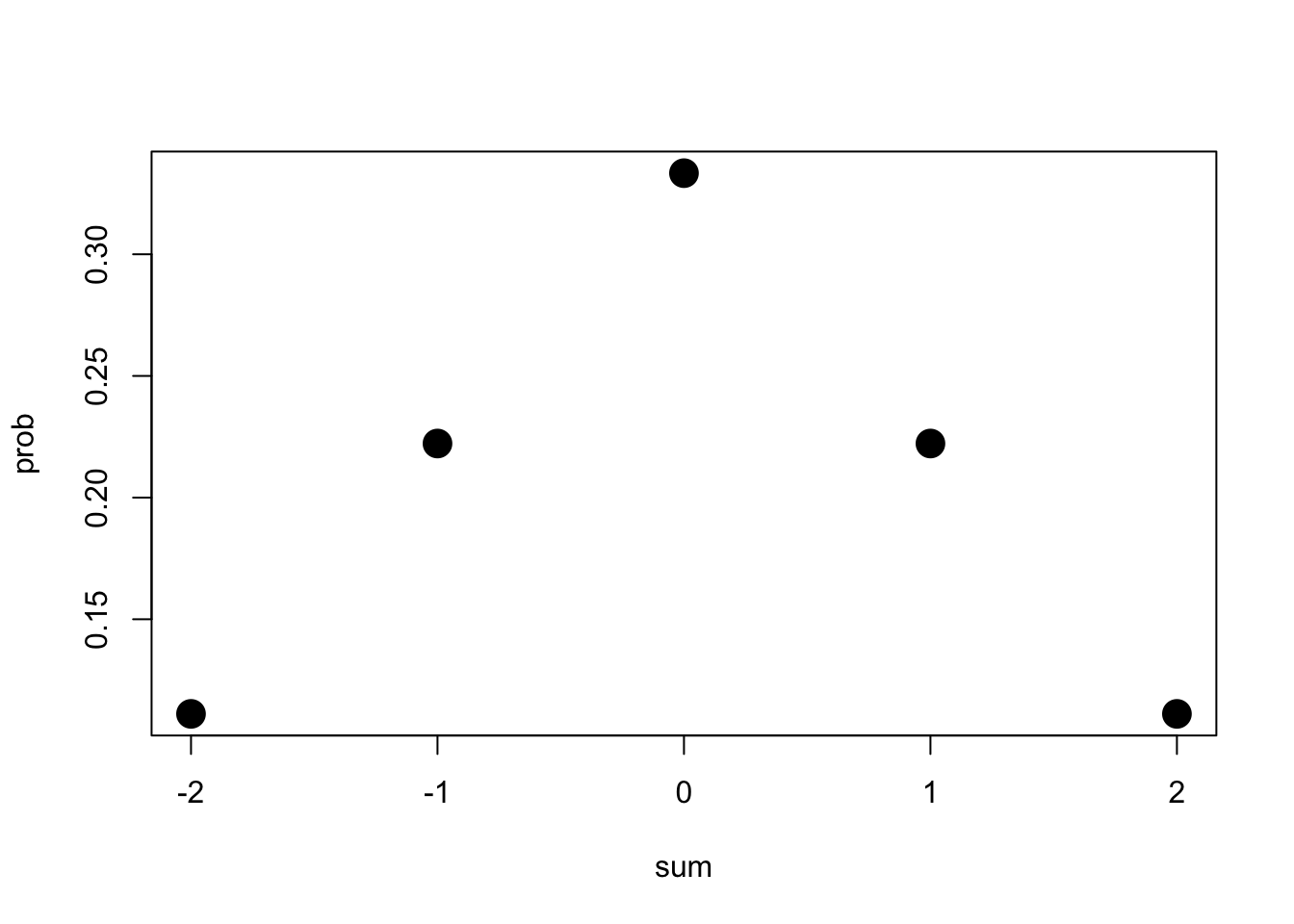 Notice how the sum of two draws from X have already pulled this in closer to the mean: the least common sums are 2 and -2, and the most common is the mean (0).
Let’s do this one more time: we consider all possible sums of three \(Xs\), we will plot their distribution, and we will overlay a normal distribution with the same mean and variance as \(X_1+X_2+X_3\).
X1=rep(c(-1,0,1),9)
X2=rep(c(-1,-1,-1,0,0,0,1,1,1),3)
X3=c(rep(-1,9),rep(0,9),rep(1,9))
tab<-cbind(X1,X2,X3,sum=X1+X2+X3,prob=rep(1/3*1/3*1/3,27))
tab
## X1 X2 X3 sum prob
## [1,] -1 -1 -1 -3 0.03703704
## [2,] 0 -1 -1 -2 0.03703704
## [3,] 1 -1 -1 -1 0.03703704
## [4,] -1 0 -1 -2 0.03703704
## [5,] 0 0 -1 -1 0.03703704
## [6,] 1 0 -1 0 0.03703704
## [7,] -1 1 -1 -1 0.03703704
## [8,] 0 1 -1 0 0.03703704
## [9,] 1 1 -1 1 0.03703704
## [10,] -1 -1 0 -2 0.03703704
## [11,] 0 -1 0 -1 0.03703704
## [12,] 1 -1 0 0 0.03703704
## [13,] -1 0 0 -1 0.03703704
## [14,] 0 0 0 0 0.03703704
## [15,] 1 0 0 1 0.03703704
## [16,] -1 1 0 0 0.03703704
## [17,] 0 1 0 1 0.03703704
## [18,] 1 1 0 2 0.03703704
## [19,] -1 -1 1 -1 0.03703704
## [20,] 0 -1 1 0 0.03703704
## [21,] 1 -1 1 1 0.03703704
## [22,] -1 0 1 0 0.03703704
## [23,] 0 0 1 1 0.03703704
## [24,] 1 0 1 2 0.03703704
## [25,] -1 1 1 1 0.03703704
## [26,] 0 1 1 2 0.03703704
## [27,] 1 1 1 3 0.03703704tab1=aggregate(prob~sum,data=tab,sum)
tab1## sum prob
## 1 -3 0.03703704
## 2 -2 0.11111111
## 3 -1 0.22222222
## 4 0 0.25925926
## 5 1 0.22222222
## 6 2 0.11111111
## 7 3 0.03703704mean<-sum(tab1[,1]*tab1[,2])
var<-sum(tab1[,1]^2*tab1[,2])
{plot(tab1,pch=19,cex=2,ylim=c(0,.3))
curve(dnorm(x,mean,sqrt(var)),add=T)} Remarkably similar! The distribution of the sum of three draws of
\[ X=\left\{\begin{matrix} 1& \text{with probability 1/3} \\ 2 & \text{with probability 1/3} \\ 3 & \text{with probability 1/3} \end{matrix}\right\}\]
is eerily close to normal. Notice here that we didn’t have to divide our variance by \(\sqrt{n}\) because we were dealing with the distribution of the sum, not an average! Here’s what the distribution of \(\sum_{i=1}^4 X_i\) looks like, in case you aren’t convinced.
Remarkably similar! The distribution of the sum of three draws of
\[ X=\left\{\begin{matrix} 1& \text{with probability 1/3} \\ 2 & \text{with probability 1/3} \\ 3 & \text{with probability 1/3} \end{matrix}\right\}\]
is eerily close to normal. Notice here that we didn’t have to divide our variance by \(\sqrt{n}\) because we were dealing with the distribution of the sum, not an average! Here’s what the distribution of \(\sum_{i=1}^4 X_i\) looks like, in case you aren’t convinced.
X1=rep(c(-1,0,1),27)
X2=rep(c(-1,-1,-1,0,0,0,1,1,1),9)
X3=rep(c(rep(-1,9),rep(0,9),rep(1,9)),3)
X4=c(rep(-1,27),rep(0,27),rep(1,27))
tab<-cbind(X1,X2,X3,X4,sum=X1+X2+X3+X4,prob=rep(1/3*1/3*1/3*1/3,81))
tab1=aggregate(prob~sum,data=tab,sum)
mean<-sum(tab1[,1]*tab1[,2])
var<-sum(tab1[,1]^2*tab1[,2])
{plot(tab1,pch=19,cex=2,ylim=c(0,.3))
curve(dnorm(x,mean,sqrt(var)),add=T)}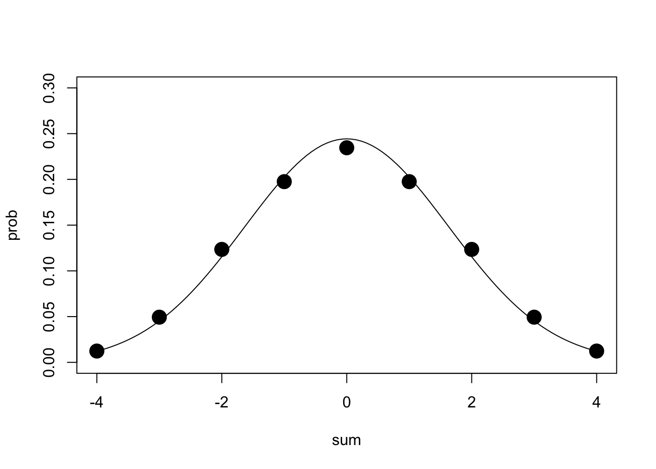
That was for a discrete probability distribution, but how about a continuous one. Imagine that every number between -1 and 1 is equally likely to be chosen—that is, imagine that our observations \(X_i \sim Uniform(-1,1)\), which looks like
curve(dunif(x,-1,1),xlim=c(-2,2))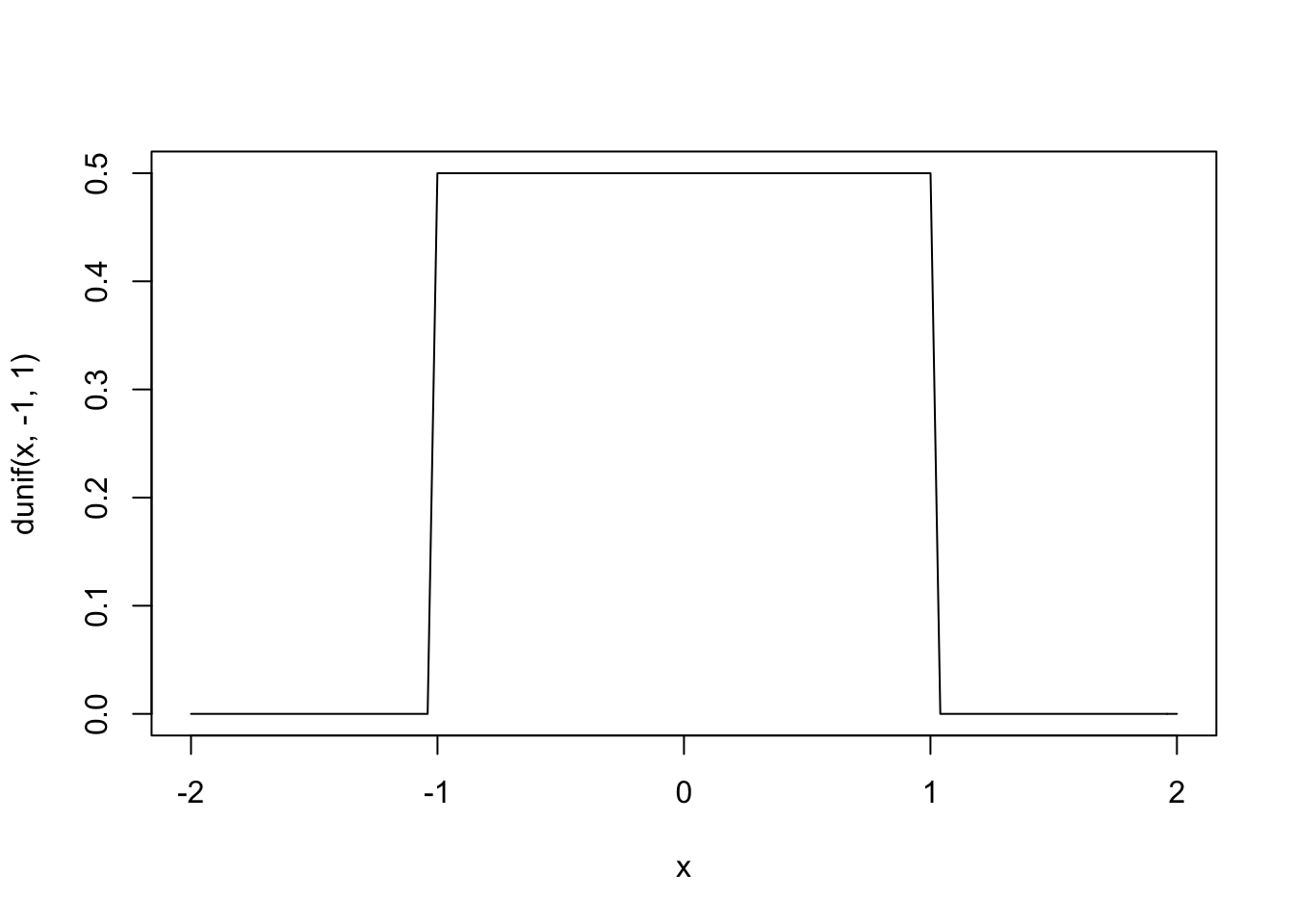 Now let’s repeatedly draw two random numbers \(X\) from this distribution, add them together, and plot the result. We will also overlay a normal distribution, \(N(0,\sqrt{4/12})\), because the variance of a uniform is given by\(\frac{1}{12}(max-min)^2\)
{hist(replicate(10000,sum(runif(2,-1,1))),breaks=100,main="",prob=T)
  curve(dnorm(x,0,sqrt(2/3)),add=T)}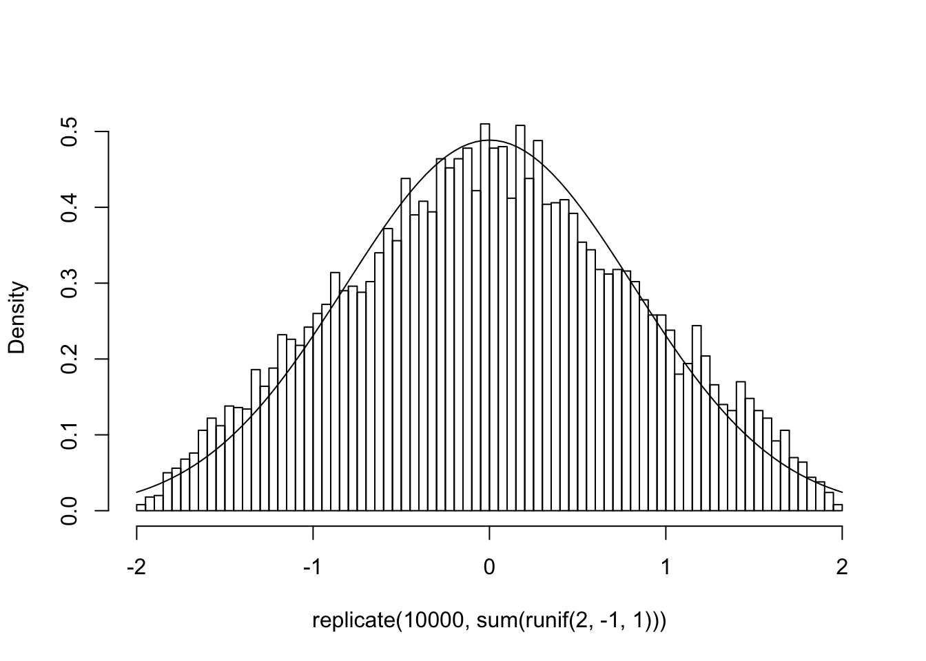
I think you get the idea, but let’s go overboard do the same for sums of larger sample sizes: how about \(n=3,5,10\)?
{par(mfrow=c(1,3))
hist(replicate(10000,sum(runif(3,-1,1))),breaks=50,main="",prob=T)
curve(dnorm(x,0,1),add=T,col="red")
hist(replicate(10000,sum(runif(5,-1,1))),breaks=50,main="",prob=T)
curve(dnorm(x,0,sqrt(5/3)),add=T,col="red")
hist(replicate(10000,sum(runif(10,-1,1))),breaks=50,main="",prob=T)
curve(dnorm(x,0,sqrt(10/3)),add=T,col="red")}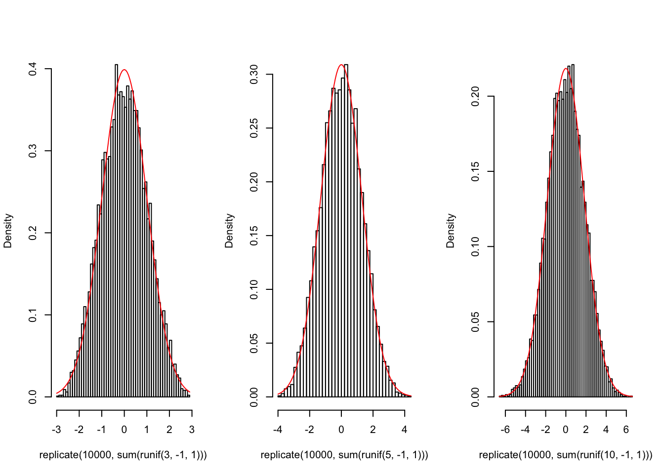
Pretty incredible, right?
Here’s a gif illustrating this exact situation—the sampling distribution of \(\sum{X_{i=1}^n} X_i, \ \ X_i \sim U(-1,1)\) for \(i=1,2,...9\).

Putting it all together, we can say that regarless of how \(X\) is distributed, as the sample size \(n\) increases, the means of the samples (the sampling distribution of \(\bar{X_n}\)) will approach this normal distribution \(N(\bar{X},\frac{\sigma^2}{\sqrt{n}})\), or equivalently, \[{\sqrt {n}}\left(\left({\frac {1}{n}}\sum _{i=1}^{n}X_{i}\right)-\mu \right)\ {\xrightarrow\ N\left(0,\sigma ^{2}\right)}\]
Finally, Back to Heights: How (Un)Sure Are We?
Going back to our very first sample of size 10, we can now say that we are 95% sure that the population mean is within \(\bar{X}\pm 1.96*\sigma/\sqrt{n}\), which is
mean(s10)+c(-1.96*pop.sd/sqrt(10),1.96*pop.sd/sqrt(10))## [1] 66.33545 71.21955But here we are using our knowledge of the population mean, 3.94 to put a confidence interval around our esimated mean! In the real world, we won’t know the mean \(\mu\) or the standard devation \(\sigma\) of the population: we will have to estimate them both, using the sample mean \(\bar{X} =\frac{1}{n}\sum_{i=1}^{n}X_i\) and the sample standard deviation \(s\). But as we will see, there’s a problem.

This works when the sample size (the “number of experiments”) is large enough, but not when it is small.
But this post is growing much too long! In the next one, we will look at how this issue was settled in the 1908 paper excerpted above (hint: the author is STUDENT).