
Enemy Tank Problem: Estimating Population Size
In wartime, it is advantageous to know how well-equipped your adversary is. Ideally, you would like to have full knowledge of their armory: exactly how many tanks, planes, and ships they have that are currently battle-ready.
Unfortunately, there is no good way to get this information. Imagine, however, that you have managed to capture \(k\) tanks from the enemy. Furthermore, each enemy tank has a serial number stamped on it. Represent the sample of serial numbers as \(\{x_1, x_2,\dots,x_k\}\). For now, we will assume that the first tank produced had the serial number \(1\), while the last tank produced has the serial number \(N\) (they don’t have to start at one, but let’s assume they do for now). It is this \(N\) that we would like to know, since that would tell us how many tanks have been produced so far. In our set of \(k\) captured enemy tanks, the largest serial number is \(m\).
So the goal is to estimate \(N\) given that we know \(k\) and \(m\). How could we use these two pieces of information (really, sample statistics) to come up with an estimator for the population parameter (i.e., the true maximum)? It seems unlikely that we would end up with a scenario where the largest serial number in our sample happens to be the largest serial number produced (where \(m=N\)), so we should guess something bigger than \(m\). Also, it seems like as the number of captured tanks \(k\) grows, \(m\) should get closer to \(N\): in the limit, the sample size would equal the population size, and so their maxima would be the same. Let’s make up an estimator for \(N\) and see how it fares (we will derive the best unbiased estimator below). Let’s use this:
\[ \widehat N = \frac{2m}{k} \]
Our estimate is always larger than \(m\), and as \(k\) grows, our estimator \(\widehat N\) shrinks. Let’s conduct a simulation to see how well this works. Let’s say the true number of tanks produced, \(N\), is \(1000\) (we don’t know this). From this population, let’s say we captured 10 tanks:
tanks=1:1000
n=max(tanks)

samp=sample(tanks,size=10, replace = F)
m=max(samp)
k=length(samp)

nhat=2*m/k
The maximum value of our sample is 1000, and so our estimator \(\widehat N\) is 198.2. Let’s do this 5000 times, taking a new sample of tanks each time.
nhats<-replicate(5000,{samp=sample(tanks,size=10, replace = F)
           m=max(samp); k=length(samp); nhat=2*m/k})

mean(nhats)
## [1] 182.2741This is not very good! Under replication, our made-up estimator is way underestimating the true \(N=1000\).
Let’s try to derive a better \(\widehat N\). We could start with the assumption that captured tank serial numbers follow a uniform distribution. This means that the serial numbers are equally spaced and that each tank serial number has an equal probability of being chosen. To take a simple example, if there were 1000 tanks in all, each tank would have a \(1/1000\) chance of being captured (assuming tanks appear randomly, which is not necessarily very likely). But we don’t know how many tanks there are in all: this is what we are trying to estimate!
One way to think about this is, what is the probability of getting a sample of serial numbers with a maximum value less than or equal to \(m\) (i.e., \(max(x)\le m\)) when the population maximum (i.e., the true total of tanks produced) is \(N\)?
In other words, how many ways are there to construct a sample of size \(k\) with a maximum no greater than the one we observed, \(m\)? Well, there are \(m\) possibilities for the first choice, \(m-1\) possibilities for the second choice (since we already used up one value: we are sampling without replacement), and so on, giving
\[ \frac{m!}{(m-k)!}=m(m-1)(m-2)\dots(m-k+1) \]
Similarly, how many ways are there to construct a sample of size \(k\) with a maximum no greater than \(N\), the number we are trying to estimate?
Well, there are \(N\) possibilities for the first captured tank \(x_1\), \(n-1\) possibilities for the second captured tank, \(n-2\) possibilities for the third tank, and so on through our last captured tank \(k\). Thus, we have
\[ \frac{N!}{(N-k)!}=N(N-1)(N-2)...(N-k+1) \]
The probability of obtaining sample \(\{x_1,\dots,x_k\}\) with \(max(x)\le m\) is thus
\[ P(max(x)\le m)=\frac{m!/(m-k)!}{N!/(N-k)!}=\frac{m!(N-k)!}{n!(m-k)!} \]
Now, the smallest possible estimate for the total number of tanks is equal to the size of our sample \(k\) (since if we captured all of the tanks, the size of our sample would be equal to the largest serial number). The largest possible estimate for the total number is equal to \(N\), the true total number of tanks produced. Thus, this function is bounded by \(k\) and \(N\).
This is the distribution function of the MLE of \(N\), i.e., \(max(x)\). This tells us, for a given \(N\) and \(k\), the probability of observing a \(m=max(x)\) less than or equal to the one we observed. However, we never observe \(N\), so we treat it as a function of \(N\) with given \(m\) and \(k\).
The distribution function is plotted below as a function of \(N\) given fixed \(m\) and \(k\): We can see that 95% of the time, the population total (\(N\)) will be less than 182 given a sample max \(m\) of 100 and a sample size \(k\) of 5 tanks.
tank.fun1<-function(x,m,k){ifelse(x==m,1,prod(m:(m-k+1))/prod(x:(x-k+1)))}

tanky<-vector()
for(i in 100:350)tanky[i-99]<-tank.fun1(x=i,m=100,k=5)

ggplot(data.frame(y=tanky,x=100:350),aes(x,y))+geom_point()+theme_minimal()+ylab("Prob( max <= m)")+xlab("N")+geom_hline(aes(yintercept=.05),lty=3)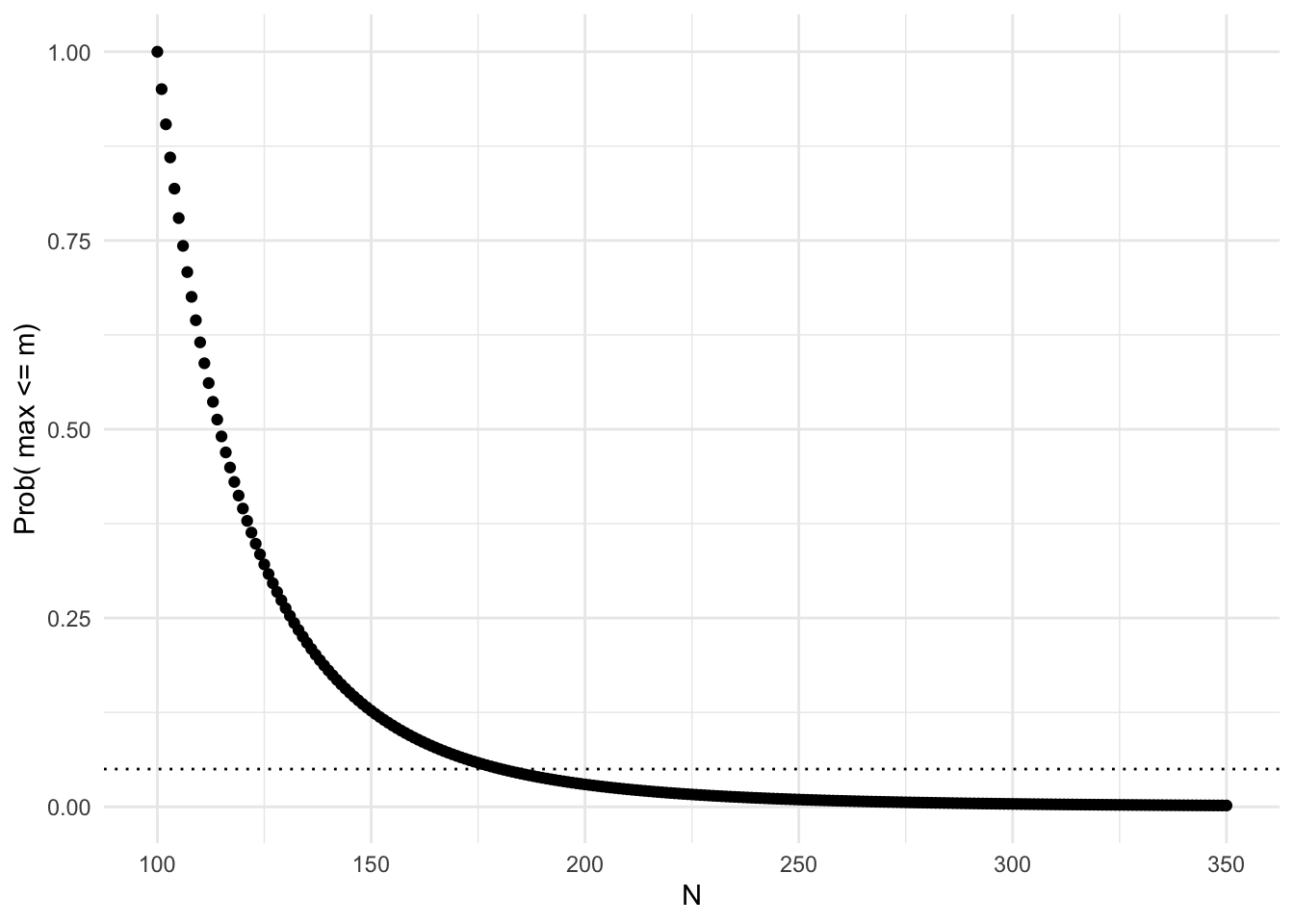
Let’s say we discover 5 more tanks. Holding everything else constant, how does this change our distribution function?
tanky1<-vector()
for(i in 100:350)tanky1[i-99]<-tank.fun1(x=i,m=100,k=10)

ggplot(data.frame(y=tanky1,y1=tanky,x=100:350),aes(x,y))+geom_point()+geom_point(aes(x,y1),color="gray")+theme_minimal()+ylab("Prob( max <= m)")+xlab("N")+geom_hline(aes(yintercept=.05),lty=3)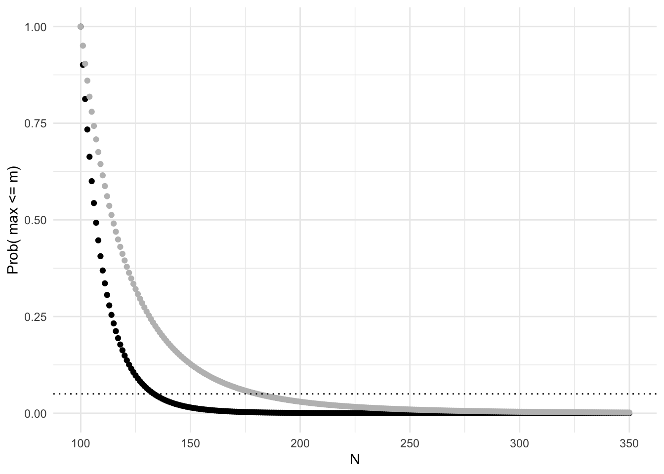
Now 95% of the time we expect the total population to be less than or equal to 135 (where black curve crosses dotted line; gray curve is from the previous plot where \(k=5\)). This makes sense: increasing the sample size should result in a more precise estimate of N, thus bringing \(m\) closer.
But what is our best guess about \(N\)? We could just take the median (fiftieth percentile) from the distribution functin above: for the sample size of 5, we get an estimate of approximately 116. But is that the best estimate we can produce?
Assuming we draw a sample of \(k\) tanks from a total of \(N\) tanks, we can compute the probability that the largest serial number in the sample will be equal to \(m\).
First, we need the total number of possible samples of size \(k\) from the total \(N\), which is just \({n \choose k}=\frac{n!}{(N-k)!k!}\).
Now, each of these samples has a sample maximum: we want to know how many of these samples have a maximum of \(m\). If \(m\) has to be the sample maximum, then one of our \(k\) tanks is fixed at \(m\) and all of the other \(k-1\) tanks must have smaller serial numbers (\(m-1\) or less). Thus, the number of samples of size \(k\) where the maximum is \(m\) is \({m -1 \choose k-1}=\frac{m-1!}{(m-k-2)!(k-1)!}\).
So we can say, out of all possible samples of size \(k\), the proportion of those with a maximum of \(m\) is \(p(m)={m -1 \choose k-1}/{N \choose k}\). Not surprsingly, this is the derivative of the distribution function above with respect to m (but I won’t show this here)!
tank.fun2<-function(x,m,k){choose(m-1,k-1)/choose(x,k)}

tanky2<-vector()
for(i in 100:350)tanky2[i-99]<-tank.fun2(i,100,5)
qplot(y=tanky2,x=100:350)+geom_line()+theme_minimal()+ylab("Prob( max = m)")+xlab("N")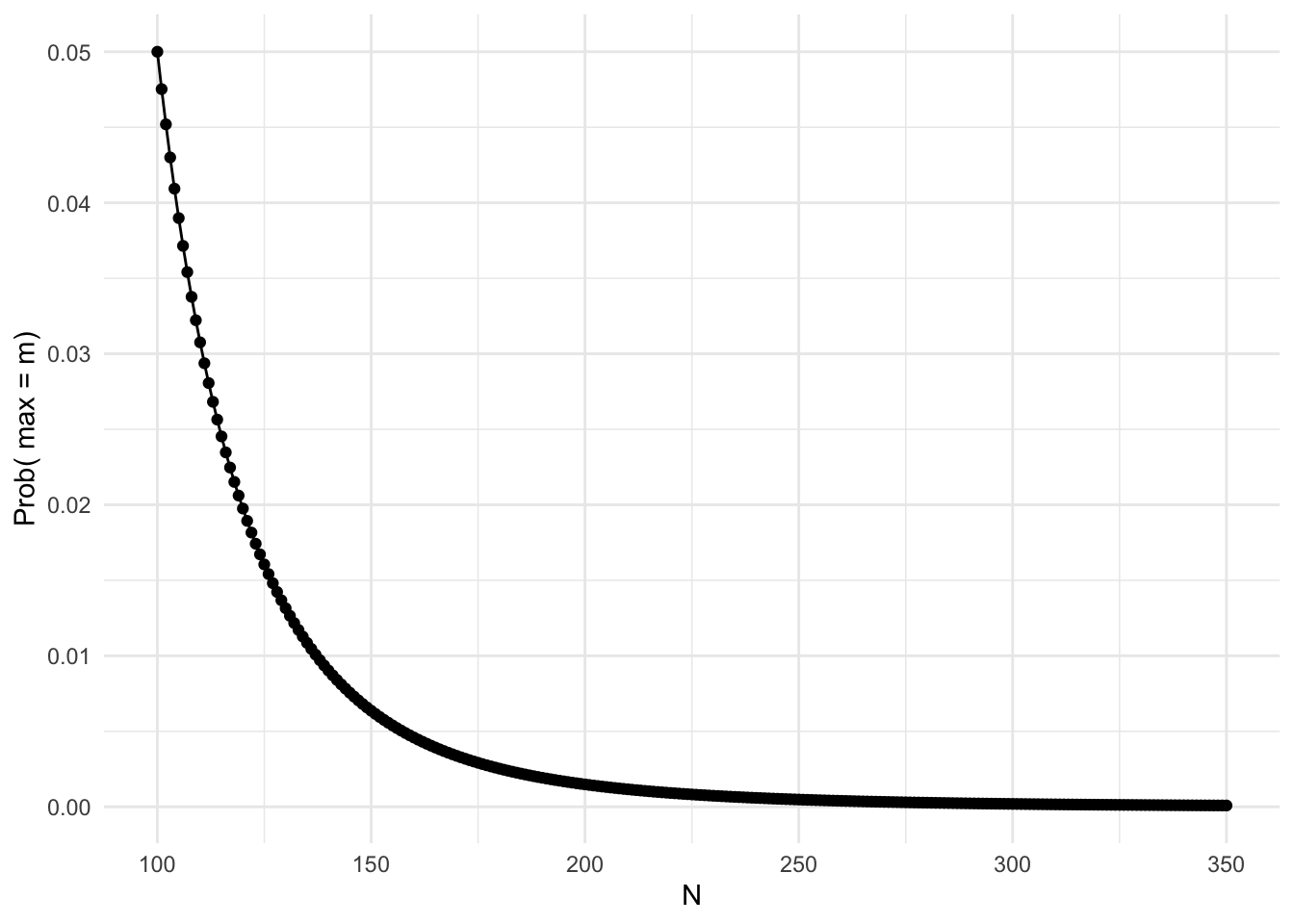
#tanky2Notice that the value of \(N\) that maximizes the probability is just our sample maximum \(m\). This seems odd: 100 seems almost certain to underestimate the true \(N\). We will see below that it is biased. Recall that the bias of an estimator is how much it deviates from the true value on average: We will show that \(E[m]\ne N\)
Since we have the probability distribution of the sample max \(m\), let’s find the expected value of \(m\). Recall that the expected value of a variable is just the sum of the values the variable takes on, weighted by their probability. That is, \(E(x)=\sum_i x_i\cdot p(x_i)\). The smallest possible value of \(m\) is \(k\) (the number of tanks in the sample), and the largest possible value is \(N\) (the number we are trying to estimate), so the expected value is
\[ \begin{aligned} E[m]&=\sum_{m=k}^N m\cdot p(m)\\ &=\sum_{m=k}^N m\cdot{m -1 \choose k-1}/{N \choose k}\\ &=\frac{1}{N\choose k}\sum_{m=k}^N m\cdot \frac{(m-1)!}{(m-k)!(k-1)!}\\ &=\frac{1}{{N\choose k}(k-1)! }\sum_{m=k}^N \frac{m!}{(m-k)!}\\ &=\frac{k!}{(k-1)!}\frac{1}{{N\choose k}}\sum_{m=k}^N {m \choose k}\\ &=k\frac{{N+1 \choose k+1}}{{N\choose k}}\phantom{xxxxxxxxxxxxxxxxx} ^* since \sum_{m=k}^N {N\choose k} = {N+1 \choose k+1} \\ &=k\frac{N+1}{k+1} \end{aligned} \] 1
Now, so we have \(E[m]=\frac{k(N+1)}{k+1}\). This estimator is biased, since \(E[m]-N=\frac{k-N}{k+1}\). Solving for N, we get
\[ \begin{aligned} E[m]&=\frac{k(N+1)}{k+1}\\ N+1&=\frac{E[m](k+1)}{k}\\ N&=E[m](1+\frac{1}{k})-1\\ \end{aligned} \]
If we use \(\widehat{N}=m(1+\frac{1}{k})-1\) instead, we have an unbiased estimator: \[ \begin{aligned} E[\widehat N]&=E[m(1+\frac{1}{k})-1]\\ &=(1+\frac{1}{k})E[m]-1\\ &=(1+\frac{1}{k})\frac{k(N+1)}{k+1}-1\\ &=(\frac{k+1}{k})\frac{k(N+1)}{k+1}-1\\ &=N \end{aligned} \] \(\widehat{N}\) is actually the minimum-variance unbiased estimator, but I won’t show this now!
Using our unbiased estimator, we get
\[ \begin{aligned} \widehat N&=m(1+\frac{1}{k})-1\\ &= 100(1+\frac1 5)-1\\ &=100+20-1\\ &=119 \end{aligned} \] Notice what is going on here with the \(100+20-1\). We are taking the sample maximum 100 and adding to the average gap between the numbers in the sample. The average gap between numbers in the sample is \(\frac{m-k}{k}=\frac{100-5}{5}=19\) (we subtract \(k\)) from the top because the numbers themselves should not be included in the gap.
Comparison Simulation
Let’s do another simulation to see all of this in action.
Say the enemy has actually produced \(N=250\) tanks (we obviously don’t know this) and we capture \(k=5\) of them.
tanks=1:250
n=max(tanks)

samp=sample(tanks,size=5, replace = F)
m=max(samp)
k=length(samp)

nhat=m+(m/k)-1
The maximum value of our sample is 250, and so our estimator \(\widehat N\) is 285.8. Let’s do this 5000 times, taking a new sample of tanks each time.
nhats<-replicate(5000,{samp=sample(tanks,size=5, replace = F)
           m=max(samp); k=length(samp); nhat=m+(m/k)-1})

mean(nhats)
## [1] 250.0882dists<-replicate(5000,{mean(abs(diff(sort(sample(1:100,5, replace = T)))))})The average of these 5000 estimates is pretty close to 250. But look at the distribution:
qplot(nhats)+theme_minimal()
runavg<-vector()
for(i in 1:5000) runavg[i]<-mean(nhats[1:i])
qplot(1:5000,runavg)+geom_line()+geom_hline(yintercept=250,color="red")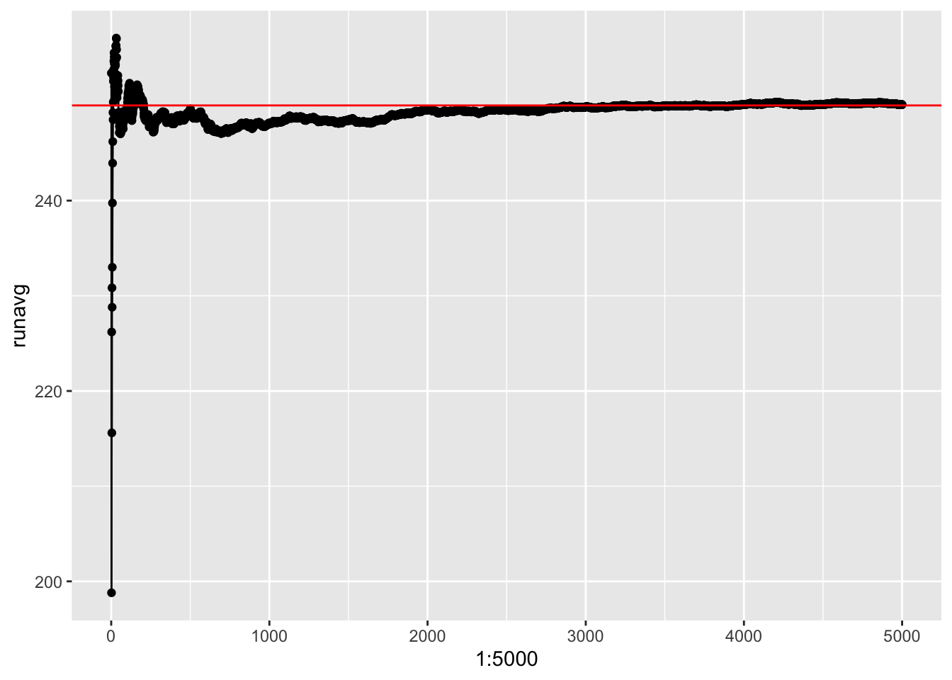
How does this compare to our median estimator?
tank.fun2<-function(x,m,k){choose(m-1,k-1)/choose(x,k)}

nhats2<-vector()
for(j in 1:5000){
samp=sample(tanks,size=5, replace = F); tanky<-vector(); m=max(samp); for(i in m:350)tanky[i-m-1]<-tank.fun1(i,m,5); nhats2[j]<-m+sum(tanky>.5)+1}

mean(nhats2)
## [1] 239.3914Here’s the distribution. Notice that the running average converges somewhere between 239 and 240 rather than 250, indicating that this estimator is biased (though not too terribly).
qplot(nhats)+theme_minimal()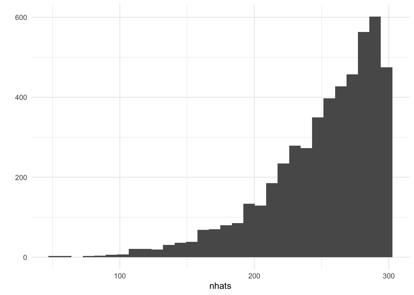
runavg<-vector()
for(i in 1:5000) runavg[i]<-mean(nhats2[1:i])
qplot(1:5000,runavg)+geom_line()+geom_hline(yintercept=runavg[5000],color="red")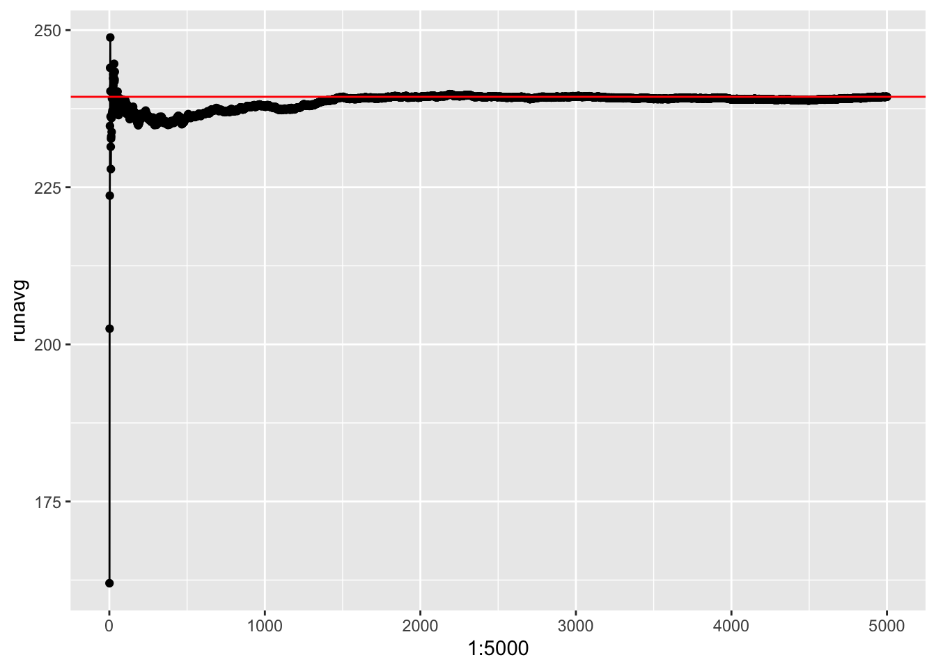
Not just tanks!
For all of our sakes, let’s hope we won’t have to actually estimate enemy tank production in real life. But there are many other applications of this! Imagine you are a manufacturer and you want to estimate the number of products produced by your competitors: all you need is a serial number (and the more, the better)! Back in 2008, a London investor solicited iPhone serial numbers from people online and was able to estimate that Apple had sold 9,190,680 iPhones to the end of September. This comes to just over 1,000,000 per month, making it very likely that Apple would sell more than 10,000,000 by year-end (indeed, they officially reported surpassing the mark in October, just as predicted by the estimate).
Takehome
Here’s a handy table for getting a rough point estimate and confidence interval (leaving out the minus one)
| k | point estimate | confidence interval |
|---|---|---|
| 1 | 2m | [m, 20m] |
| 2 | 1.5m | [m, 4.5m] |
| 5 | 1.2m | [m, 1.82m] |
| 10 | 1.1m | [m, 1.35m] |
| 20 | 1.05m | [m, 1.16m] |
Where does this come from?
Imagine we have a continuous interval from 0 to 1 inclusive. The probability that a sample of size \(k\) will have a maximum less than or equal to \(m\), where \(m\) is some number \(0 \le m \le 1\), is \(m^k\). For example, if \(m=0.5\), the probability that all the \(k\) numbers in your sample are less than or equal to \(0.5\) is just \[\underbrace{0.5*0.5...*0.5}_{k\ times}=0.5^k=m^k=p(M\le m)=F_M(m)\]
ggplot(data.frame(m=c(0, 1)), aes(m)) +
  stat_function(fun=function(x) x^3)+ylab('p(M <= m)')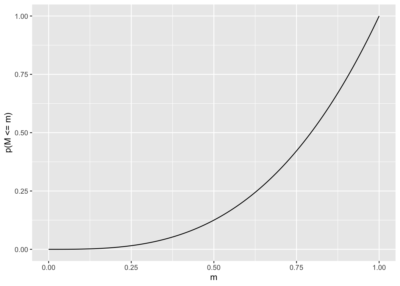
Here, \(F_M(m)=p(M\le m)=m^k\) is the CDF of the sample max \(M\), the function that returns the probability that the sample max is less than or equal to some value \(m\). The quantile function is given by the inverse of this CDF, i.e., \(F^{-1}_M(m)\). This tells you what sample max \(m\) would make \(F_M(m)\) return a certain probability \(p\). (This is just like when you look up \(p=.5\) z-table and it gives you \(z=0\): \(InvNorm(p=.5)=0\).)
Now, in our case \(F_M(m)=m^k=p, so\ \ F^{-1}_M(m)=p^{1/k}\). So for a population maximum of \(N\), we are \(95%\) confident that the sample maximum is covered by the interval
\[ .025^{1/k}N\le m \le .975^{1/k}N \] (We multiply by \(N\) here to take the interval from \([0,1]\) to \([O,N]\).) Solving for N in the middle gives
\[ \begin{aligned} .025^{1/k}\frac 1 m &\le \frac 1 N \le .975^{1/k}\frac 1 m\\ \frac{m}{.025^{1/k}} &\ge N \ge \frac{m}{.975^{1/k}}\\ \frac{m}{.975^{1/k}} &\le N \le \frac{m}{.025^{1/k}}\\ \end{aligned} \]
Giving the population max \(N\) a \(95%\) CI of \([\frac{m}{.975^{1/k}}, \frac{m}{.025^{1/k}}]\). Thus, if you just have a single observation \(k\), your \(95%\) CI is \([\frac{m}{.975}, \frac{m}{.025}]\) or \([1.026 m, 40m]\). Since the sampling distribution is asymmetrical, we are better off reporting the asymmetric \(95%\) CI by doing \([\frac{m}{1}, \frac{m}{.05^{1/k}}]\). This yields \([m, 20m]\) for a single sample (these values are reported above).
References:
en.wikipedia.org/wiki/German_tank_problem mathsection.com/german-tank-problem
This is the hockey-stick identity from pascal’s triangle, but we can derive it easily here from \(p(m)\). Since \(p(m)={m -1 \choose k-1}/{N \choose k}\) must sum to 1 (it is a probability mass function),\(1=\sum_{m=k}^N{m -1 \choose k-1}/{N \choose k} \implies \sum_{m=k}^N{m -1 \choose k-1}= {N \choose k}\)}↩