
Why do we use sample means?
The sample mean, \(\bar x = \frac 1 N\sum x_i\), is a workhorse of modern statistics. For example, t tests compare two sample means to judge if groups are likely different at the population level, and ANOVAs compare sample means of more groups to achieve something similar. But does \(\bar x\) actually deserve the great stature is has inherited?
I recently heard a talk by Dr. Clintin Davis-Stober at the 2018 Psychonomics Annual Meeting that was really fun, and got me thinking about this question. For a preprint of a relevant paper, see here
Let’s assume we have four groups, A, B, C, and D, and we want to estimate the true difference between the groups. Assume there is a true difference between groups of 0.5 (group B is slightly higher).
Stein’s Paradox and Regularization Estimators
Though the sample mean is unbiased, Stein (1956) showed that better accuracy could be obtained using biased estimators. This result lead to many modern techniques (including lasso/ridge regression).
Let’s assume we have four groups, A, B, C, and D, and we want to estimate the true difference between the groups. Assume there is a true difference between groups of 0.5 (group A is slightly lower than group B, which is in turn slightly lower that group C, which is in turn slightly lower than group D).
popA=rnorm(10000,mean=0,sd = 4)
popB=rnorm(10000,mean=0.5,sd = 4)
popC=rnorm(10000,mean=1.0, sd = 4)
popD=rnorm(10000,mean=1.5, sd = 4)


A=sample(popA, 10)
B=sample(popB, 10)
C=sample(popC, 10)
D=sample(popD, 10)


dat<-data.frame(A,B,C,D)
#dat<-read.csv("dat.csv")
#dat$X<-NULL
dat1<-gather(dat,key = group)
dat1$true<-c(rep(0,10),rep(.5,10),rep(1,10),rep(1.5,10))
dat1$samp.mean<-c(rep(mean(A),10),rep(mean(B),10),rep(mean(C),10),rep(mean(D),10))

ggplot(dat1,aes(y=value,x=group,color=group))+geom_point()+scale_x_discrete()+geom_hline(aes(yintercept = true,color=group),lty=2)+geom_point(aes(x=group,y=samp.mean),pch=8,size=3)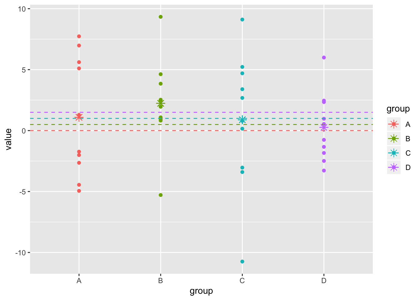
The traditional approach would be to find the sample means of the groups, call them \(\bar x_A, \bar x_B, \bar x_C, \bar x_D\) (colored asterisks, above), and find the differences between them.
Stein’s Paradox reveals that this approach is suboptimal, because each sample mean is isolated from the others. If instead you took into account information from the other groups and “shrunk” your estimates toward the grand mean, you would achieve greater overall accuracy.
It’s only paradoxical because the groups don’t have to have anything to do with each other. Davis-Stober, Dana, and Rouder (2018) relate an example
…the goal is to measure the true mean of three populations: the weight of all hogs in Montana, the per-capita tea consumption in Taiwan, and the height of all redwood tress in California. These values could be estimated separately by getting a sample of hogs, a sample of Taiwanese households, and a sample of redwood trees and using each sample mean as an estimate of the corresponding population mean… the total error of these three estimates is expected to be reduced if, rather than using sample means to estimate each individual population mean, scale information from all three samples is pooled. To be clear, pooling only helps in overall estimation—hog weight information does not reduce the error of the redwood tree heights estimate. Rather, pooling will leave some individual estimates worse off (say hog weight) with other individual estimates better off, and the gains outweigh the losses on balance.
Let’s demonstrate this by comparing the accuracy of different estimators, measuring accuracy using root-mean-square error (RSME) between the measured values and the true values, i.e.,
\[ RMSE=\sqrt{\frac 1 K\sum_i^K{(\widehat \mu_i- \mu_i)^2}} \]
Here, the RMSE for sample means is
dat1%>%group_by(group)%>%summarize(sampmean=mean(value))%>%summarize(RMSE=sqrt(mean((sampmean-c(0,.5,1,1.5))^2)))## # A tibble: 1 x 1
## RMSE
## <dbl>
## 1 1.20Made up shrinkage estimator
If we use some kind of shrinkage estimator to combine individual and pooled averages, say \(\widehat \mu=w_i\bar x_i+(1-w_i)\bar x_\cdot\) where \(\bar x_\cdot\) denotes the overall mean, do we see the expected improvement? Let’s set \(w=.8\) just for fun.
w=.8
dat1$shrinkmean<-w*dat1$samp.mean+(1-w)*mean(dat1$samp.mean)

ggplot(dat1,aes(y=value,x=group,color=group))+geom_point()+scale_x_discrete()+geom_hline(aes(yintercept = true,color=group),lty=2)+geom_point(aes(x=group,y=samp.mean),pch=8,size=3)+geom_point(aes(x=group,y=shrinkmean),pch=8,size=3,color="black")+geom_hline(aes(yintercept=mean(dat1$value)))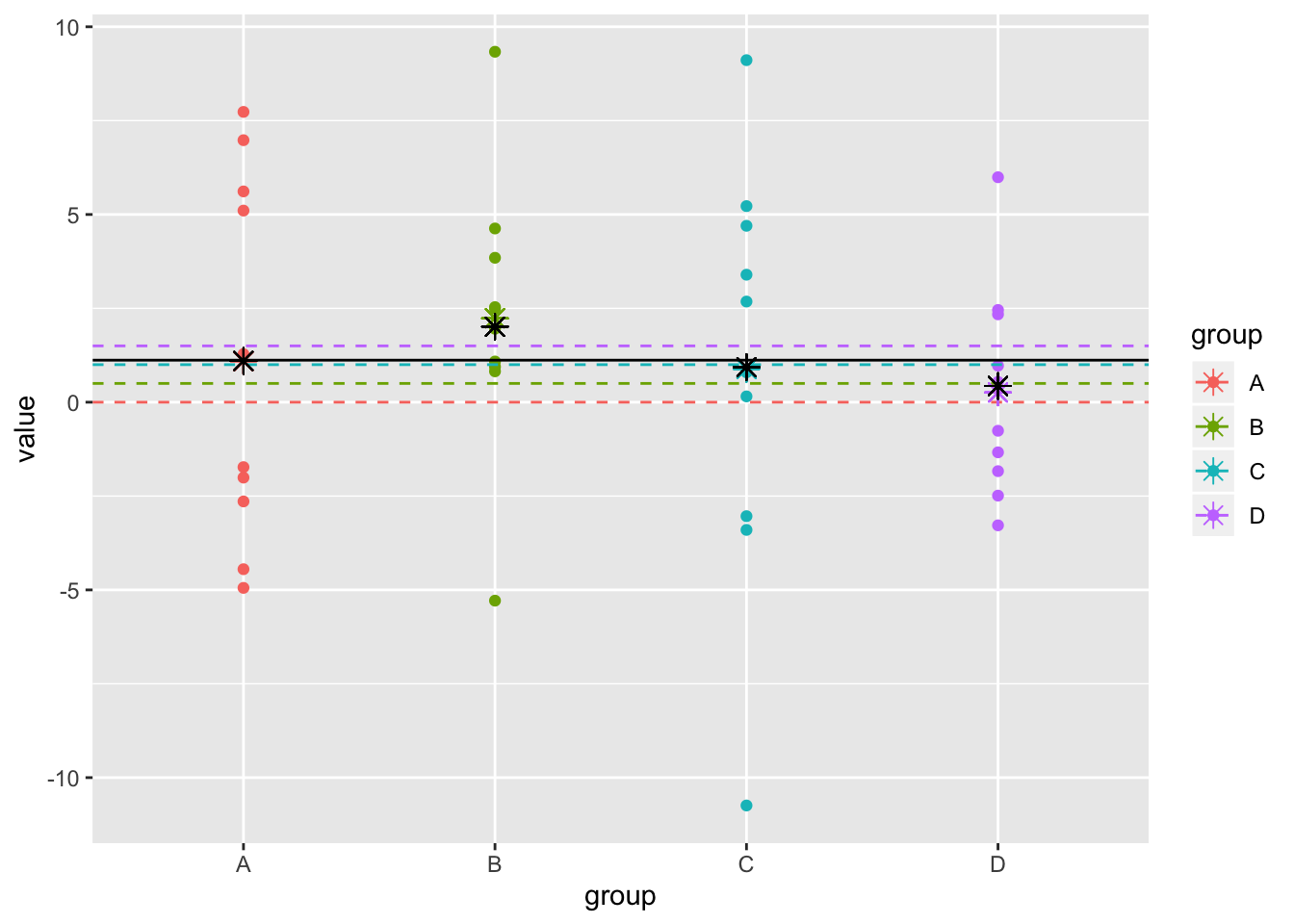
The black line represents the grand mean and the colored asterisks represent the group means. The black asterisks represent the shrinkage estimators for each group. The distance from the dashed lines (the true means) is what it’s all about!
shrinkest<-dat1%>%group_by(group)%>%summarize(shrinkest=unique(shrinkmean))%>%.$shrinkest
sqrt(mean((shrinkest-c(0,.5,1,1.5))^2))
## [1] 1.076894Hierarchical Bayes shrinkage estimates
We do get an RMSE improvement, but arbitrarily picking \(w\) is not ideal: it is better to get our shrikage estimates from a hierarchical bayesian model. Don’t worry! We will walk through this, but feel free to skip to the good stuff.
We can consider our observations to be modeled follows: \(Y_{ij}\) is the response for the \(j\)th participant in the \(i\)th group, and we use
\[ Y_{ij}=\mu+c_i+e_{ij} \] Where \(\mu\) is the grand mean, \(c_i\) is how far the mean of group \(i\) is from the grand mean, and \(e_{ij}\) is a noise parameter with mean 0 and variance \(\sigma^2\).
This is really just an ANOVA model
fit<-lm(value~group,data=dat1, contrasts=list(group=contr.sum))
summary(fit)
##
## Call:
## lm(formula = value ~ group, data = dat1, contrasts = list(group = contr.sum))
##
## Residuals:
## Min 1Q Median 3Q Max
## -11.6302 -2.7673 0.0476 2.4210 8.2231
##
## Coefficients:
## Estimate Std. Error t value Pr(>|t|)
## (Intercept) 1.1192 0.6898 1.622 0.113
## group1 -0.0256 1.1948 -0.021 0.983
## group2 1.1161 1.1948 0.934 0.356
## group3 -0.2314 1.1948 -0.194 0.848
##
## Residual standard error: 4.363 on 36 degrees of freedom
## Multiple R-squared: 0.02888, Adjusted R-squared: -0.05205
## F-statistic: 0.3569 on 3 and 36 DF, p-value: 0.7844Let’s give \(\mu\) and \(c_i\) their own prior distributions. Specifically, assume both are normal, with mean zero and and separate variance hyperparameters.
\[ \mu \sim N(0,\sigma_{\mu}^2) \\ c_i\sim N(0,\sigma_{c}^2) \]
y<-data.frame(dat)

library(rjags)

modelstring<-"model{
  for(j in 1:4){
    for(i in 1:10){
       y[i,j]~dnorm(mean+dist[j],tau)
    }
  }
mean~dnorm(0,1)
for(j in 1:4){dist[j]~dnorm(0,1)}
tau~dgamma(1,.0001)
}"


model <- jags.model(textConnection(modelstring), data = list(y = y), n.chains = 3, n.adapt= 10000)
## Compiling model graph
## Resolving undeclared variables
## Allocating nodes
## Graph information:
## Observed stochastic nodes: 40
## Unobserved stochastic nodes: 6
## Total graph size: 53
##
## Initializing modelupdate(model, 10000); # Burnin for 10000 samples
mcmc_samples <- coda.samples(model, variable.names=c("mean","dist", "tau"), n.iter=20000)
print(summary(mcmc_samples)$statistics)## Mean SD Naive SE Time-series SE
## dist[1] 0.15392124 0.83049116 3.390466e-03 3.727025e-03
## dist[2] 0.56946392 0.83284712 3.400084e-03 3.707196e-03
## dist[3] 0.08402375 0.83141159 3.394224e-03 3.724341e-03
## dist[4] -0.14371737 0.83187105 3.396099e-03 3.709378e-03
## mean 0.65681952 0.64023722 2.613758e-03 3.358874e-03
## tau 0.05765514 0.01285363 5.247472e-05 5.435118e-05shrink_ests<-summary(mcmc_samples)$statistics[,1]
shrinkmean<-shrink_ests[1:4]+shrink_ests[5]The RMSE for the shrinkage estimator is
sqrt(mean((shrinkmean-c(0,.5,1,1.5))^2))## [1] 0.7459755ggplot(dat1,aes(y=value,x=group,color=group))+geom_point()+scale_x_discrete()+geom_hline(aes(yintercept = true,color=group),lty=2)+geom_point(aes(x=group,y=samp.mean),pch=8,size=3)+geom_point(aes(x=group,y=shrinkmean),pch=8,size=3,color="black")+geom_hline(aes(yintercept=mean(dat1$value)))
Doing better than sample means with random noise!
The point of this write-up is that sometimes you can do better than sample means by using an estimator based on random noise.
For each condition, we begin by drawing a random number from a uniform distribution, say \(U(-1,1)\), call them \(u_1, u_2, u_3, u_4\).
Now, let us define our random estimator for the true mean \(\mu_i\) for group \(i\) as
\[ \hat \mu_i = \bar{x_\cdot}+b+u_i \] Where \(\bar x_\cdot\) is the grand mean, the \(u_i\) are the random draws defined above, and \(b\) is defined as follows: \(b=\frac{p-\sqrt{(p(p-1)})}{\sqrt{\sum u_i^2}}\sum u_i\bar x_i\), where \(p\) equals the number of groups (here, 4; see Stober, Dana, and Rouder 2018 for more details).
sampmeans<-dat1%>%group_by(group)%>%summarize(mean=mean(value))%>%.$mean
grandmean<-mean(dat1$value)
u<-runif(4,-1,1)
b=((4-sqrt(4*3))/sqrt(sum(u^2)))*sum(u*(sampmeans-grandmean))


rand_ests<-grandmean+b+u
dat1$rand_ests<-rep(rand_ests,each=10)
Lets see how this random estimator worked out:
sqrt(mean((rand_ests-c(0,.5,1,1.5))^2))## [1] 1.070817ggplot(dat1,aes(y=value,x=group,color=group))+geom_point()+scale_x_discrete()+geom_hline(aes(yintercept = true,color=group),lty=2)+geom_point(aes(x=group,y=samp.mean),pch=8,size=3)+geom_point(aes(x=group,y=rand_ests),pch=8,size=3,color="black")+geom_hline(aes(yintercept=mean(dat1$value)))
Better than our original of .892, which we get using the group means!
Simulation
Let’s repeat this RMSE calculation with the group means and with the random estimator very many times.
RMSE1<-vector()
RMSE2<-vector()

for(i in 1:5000){
A=sample(popA, 10)
B=sample(popB, 10)
C=sample(popC, 10)
D=sample(popD, 10)

sampmean=apply(data.frame(A,B,C,D),2,mean)

RMSE1[i]<-sqrt(mean((sampmean-c(0,.5,1,1.5))^2))

grandmean<-mean(c(A,B,C,D))
u<-runif(4,-1,1)
b=((4-sqrt(4*3))/sqrt(sum(u^2)))*sum(u*(sampmean-grandmean))
rand_ests<-grandmean+b+u

RMSE2[i]<-sqrt(mean((rand_ests-c(0,.5,1,1.5))^2))
}

mean(RMSE2<RMSE1)
## [1] 0.5296This means that more than half the time, the random estimator is outperforming the sample means!
It is important to realize that sample size and sample variance both affect this result. The larger the sample size (or the smaller the variance), the less of an effect shrinkage has on overall estimation accuracy.
In the present example, the effect size \(f^2=\frac{\frac 1 p\sum (\mu_i-\mu_{\cdot})^2}{\sigma^2}=\frac{R^2}{1-R^2}\) is 0.0297404
It can be shown that the minimum sample size per condition needed to ensure that the sample means are more accurate than random estimators on average is equal to
\[ n_r = \frac{\sqrt{p(p-1)}}{pf^2} \]
It can be helpful to consider values of \(f^2=.02, .15,\) and \(.35\) for small, medium, and large effects, respectively.
Thus, given an expected \(f^2=.02\) and \(p=4\) conditions, the minimum sample size is given by \(\frac{\sqrt{4(3)}}{4*.02}=43.3\) or \(44\) people per condition.